An article about neural networks in machine learning by Mohammad Mahdi Khoramabadi.

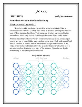
1. ‫تعالی‬ ‫باسمه‬
‫آبادی‬ ‫م‬ّ‫خر‬ ‫مهدی‬ ‫محمد‬
3981231039
Neural networks in machine learning
What are neural networks?
Neural networks, also known as artificial neural networks (ANNs) or
simulated neural networks (SNNs), are a subset of machine learning and are at the
heart of deep learning algorithms. Their name and structure are inspired by the
human brain, mimicking the way that biological neurons signal to one another.
Artificial neural networks (ANNs) are comprised of a node layers, containing an
input layer, one or more hidden layers, and an output layer. Each node, or artificial
neuron, connects to another and has an associated weight and threshold. If the
output of any individual node is above the specified threshold value, that node is
activated, sending data to the next layer of the network. Otherwise, no data is
passed along to the next layer of the network.

2. Neural networks rely on training data to learn and improve their accuracy
over time. However, once these learning algorithms are fine-tuned for accuracy,
they are powerful tools in computer science and artificial intelligence, allowing us
to classify and cluster data at a high velocity. Tasks in speech recognition or image
recognition can take minutes versus hours when compared to the manual
identification by human experts. One of the most well-known neural networks is
Google’s search algorithm.
How do neural networks work?
Think of each individual node as its own linear regression model, composed
of input data, weights, a bias (or threshold), and an output. The formula would look
something like this:
Once an input layer is determined, weights are assigned. These weights help
determine the importance of any given variable, with larger ones contributing more
significantly to the output compared to other inputs. All inputs are then multiplied
by their respective weights and then summed. Afterward, the output is passed
through an activation function, which determines the output. If that output exceeds
a given threshold, it “fires” (or activates) the node, passing data to the next layer in
the network. This results in the output of one node becoming in the input of the
next node. This process of passing data from one layer to the next layer defines this
neural network as a feedforward network.

3. Let’s break down what one single node might look like using binary values.
We can apply this concept to a more tangible example, like whether you should go
surfing (Yes: 1, No: 0). The decision to go or not to go is our predicted outcome, or
y-hat. Let’s assume that there are three factors influencing your decision-making:
Are the waves good? (Yes: 1, No: 0)
Is the line-up empty? (Yes: 1, No: 0)
Has there been a recent shark attack? (Yes: 0, No: 1)
Then, let’s assume the following, giving us the following inputs:
X1 = 1, since the waves are pumping
X2 = 0, since the crowds are out
X3 = 1, since there hasn’t been a recent shark attack
Now, we need to assign some weights to determine importance. Larger weights
signify that particular variables are of greater importance to the decision or
outcome.
W1 = 5, since large swells don’t come around often
W2 = 2, since you’re used to the crowds
W3 = 4, since you have a fear of sharks

4. Finally, we’ll also assume a threshold value of 3, which would translate to a bias
value of –3. With all the various inputs, we can start to plug in values into the
formula to get the desired output.
Y-hat = (1*5) + (0*2) + (1*4) – 3 = 6
If we use the activation function from the beginning of this section, we can
determine that the output of this node would be 1, since 6 is greater than 0. In this
instance, you would go surfing; but if we adjust the weights or the threshold, we
can achieve different outcomes from the model. When we observe one decision,
like in the above example, we can see how a neural network could make
increasingly complex decisions depending on the output of previous decisions or
layers.
In the example above, we used perceptrons to illustrate some of the
mathematics at play here, but neural networks leverage sigmoid neurons, which are
distinguished by having values between 0 and 1. Since neural networks behave
similarly to decision trees, cascading data from one node to another, having x
values between 0 and 1 will reduce the impact of any given change of a single
variable on the output of any given node, and subsequently, the output of the
neural network.
As we start to think about more practical use cases for neural networks, like
image recognition or classification, we’ll leverage supervised learning, or labeled
datasets, to train the algorithm. As we train the model, we’ll want to evaluate its
accuracy using a cost (or loss) function. This is also commonly referred to as the
mean squared error (MSE). In the equation below,

5. i represents the index of the sample,
y-hat is the predicted outcome,
y is the actual value, and
m is the number of samples.
Ultimately, the goal is to minimize our cost function to ensure correctness of
fit for any given observation. As the model adjusts its weights and bias, it uses the
cost function and reinforcement learning to reach the point of convergence, or the
local minimum. The process in which the algorithm adjusts its weights is through
gradient descent, allowing the model to determine the direction to take to reduce
errors (or minimize the cost function). With each training example, the parameters
of the model adjust to gradually converge at the minimum.

6. Types of neural networks
Neural networks can be classified into different types, which are used for
different purposes. While this isn’t a comprehensive list of types, the below would
be representative of the most common types of neural networks that you’ll come
across for its common use cases:
The perceptron is the oldest neural network, created by Frank Rosenblatt in 1958.
It has a single neuron and is the simplest form of a neural network:
History of neural networks
The history of neural networks is longer than most people think. While the
idea of “a machine that thinks” can be traced to the Ancient Greeks, we’ll focus on
the key events that led to the evolution of thinking around neural networks, which
has ebbed and flowed in popularity over the years:
1943: Warren S. McCulloch and Walter Pitts published “A logical calculus of the
ideas immanent in nervous activity (PDF, 1 MB) (link resides outside IBM)” This
research sought to understand how the human brain could produce complex
patterns through connected brain cells, or neurons. One of the main ideas that came
out of this work was the comparison of neurons with a binary threshold to Boolean
logic (i.e., 0/1 or true/false statements).

7. 1958: Frank Rosenblatt is credited with the development of the perceptron,
documented in his research, “The Perceptron: A Probabilistic Model for
Information Storage and Organization in the Brain” (PDF, 1.6 MB) (link resides
outside IBM). He takes McCulloch and Pitt’s work a step further by introducing
weights to the equation. Leveraging an IBM 704, Rosenblatt was able to get a
computer to learn how to distinguish cards marked on the left vs. cards marked on
the right.
1974: While numerous researchers contributed to the idea of backpropagation, Paul
Werbos was the first person in the US to note its application within neural
networks within his PhD thesis (PDF, 8.1 MB) (link resides outside IBM).
1989: Yann LeCun published a paper (PDF, 5.7 MB) (link resides outside IBM)
illustrating how the use of constraints in backpropagation and its integration into
the neural network architecture can be used to train algorithms. This research
successfully leveraged a neural network to recognize hand-written zip code digits
provided by the U.S. Postal Service.