Call Girls Service Nashik Vaishnavi 7001305949 Independent Escort Service Nashik
REYNOLD TRANSPORT THEOREM
1. Reynolds Transport Theorem
This theorem transforms the system formulation to control volume formulation; which
is given by the following expression
∫∫ ρ+∀ρ
∂
∂
=
∀ .S.C..C
sys
dA)n.V(bdb
tDt
DB
1. The first integral represents the rate of change of the extensive property in the
control volume.
2. The second integral represents the flux of the extensive property across the
control surface.
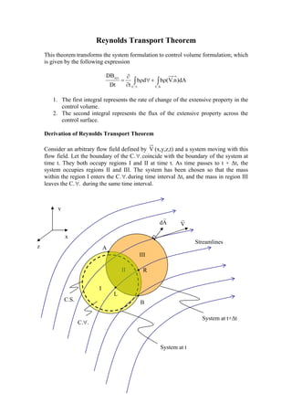
Derivation of Reynolds Transport Theorem
Consider an arbitrary flow field defined by V (x,y,z,t) and a system moving with this
flow field. Let the boundary of the C. .∀ coincide with the boundary of the system at
time t. They both occupy regions I and II at time t. As time passes to t + ∆t, the
system occupies regions II and III. The system has been chosen so that the mass
within the region I enters the C. .∀ during time interval ∆t, and the mass in region III
leaves the C. .∀ during the same time interval.
II
III
I
.
R
B
A
L
Streamlines
C.S.
System at t+∆t
System at t
C.∀.
y
z
x
Ad
r
V
r
2. Mathematically, the rate of change of B for the system is given by
t
)B()B(
lim
Dt
DB tsysttsys
0t
sys
∆
−
=
∆+
→∆ or
⎥
⎥
⎥
⎥
⎥
⎦
⎤
⎢
⎢
⎢
⎢
⎢
⎣
⎡
∆
⎟
⎟
⎠
⎞
⎜
⎜
⎝
⎛
∀ρ+∀ρ−
⎟
⎟
⎠
⎞
⎜
⎜
⎝
⎛
∀ρ+∀ρ
=
∫∫∫∫
∀∀∆+∀∀
→∆
t
dbdbdbdb
lim
Dt
DB ttt
0t
sys 2123
Since the limit of the sums equals the sum of the limits one can write,
t
db
lim
t
db
lim
t
dbdb
lim
Dt
DB t
0t
tt
0t
ttt
0t
sys 1322
∆
⎟
⎟
⎠
⎞
⎜
⎜
⎝
⎛
∀ρ
−
∆
⎟
⎟
⎠
⎞
⎜
⎜
⎝
⎛
∀ρ
+
⎥
⎥
⎥
⎥
⎥
⎦
⎤
⎢
⎢
⎢
⎢
⎢
⎣
⎡
∆
⎟
⎟
⎠
⎞
⎜
⎜
⎝
⎛
∀ρ−
⎟
⎟
⎠
⎞
⎜
⎜
⎝
⎛
∀ρ
=
∫∫∫∫
∀
→∆
∆+∀
→∆
∀∆+∀
→∆
1 2 3
Since the volume 2∀ becomes that of the C. .∀ as ∆t → 0 in the limit we have for the
1st limit expression,
∫
∫∫
∀
∀∆+∀
→∆ ∀ρ
∂
∂
=
⎥
⎥
⎥
⎥
⎥
⎦
⎤
⎢
⎢
⎢
⎢
⎢
⎣
⎡
∆
⎟
⎟
⎠
⎞
⎜
⎜
⎝
⎛
∀ρ−
⎟
⎟
⎠
⎞
⎜
⎜
⎝
⎛
∀ρ
..C
ttt
0t db
tt
dbdb
lim
22
In the 2nd
limit term the integral ∫
∀
∀
3
dbρ represents the amount of property B that has
crossed the part of C.S. (say ARB). This value divided by ∆t gives the average rate of
flux of B across ARB during the time interval ∆t. Then the limit of that term can be
written as
( )
∫
∫
ρ=
∆
⎟
⎟
⎠
⎞
⎜
⎜
⎝
⎛
∀ρ
=
∆
∆+∀
→∆
∆+
→∆
III.S.C
tt
0t
ttIII
0t dA)n.V(b
t
db
lim
t
B
lim
3
Similarly the last term represents the exact rate of influx of B into the C. .∀ at time t
through the part of C.S. (ALB). This may be written as
∫
∫
ρ=
∆
⎟
⎟
⎠
⎞
⎜
⎜
⎝
⎛
∀ρ
∀
→∆
I.S.C
t
0t dA)n.V(b
t
db
lim
1
3. The last two limiting processes represent the net flux rate of B across the entire
control surface. They can be replaced by one term as follows,
∫ ρ
.S.C
dA)n.V(b
where V is the velocity vector and n is the unit vector pointing outward from an
enclosed region.
Finally we have:
∫∫ ρ+∀ρ
∂
∂
=
∀ .S.C..C
sys
dA)n.V(bdb
tDt
DB
1 2 3
The physical meanings of the terms are:
1. The total rate of change of any arbitrary extensive property B, of the system;
2. The time rate of change of the arbitrary extensive property B within the
control volume
3. The net rate of flux of the extensive property through the control surface.
V is measured in the above equations relative to control volume which is fixed
relative to the reference coordinates x, y and z. Thus, the time rate of change of the
arbitrary extensive property B within the control volume must be evaluated by an
observer fixed in the control volume.