![Transforms
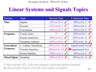
• Provide alternate signal & system representations
The Laplace Transform – SPFirst Ch. 16 Intro
Simplifies analysis in some cases
Reveals new properties (e.g. bandwidth)
H(s)
h(t)
Input-Output
Physical Model
Algebra: Poles
and Zeros
Passbands and
Stopbands
H(jw)
Input-Output
Physical Model
s = jw
Passbands and
Stopbands
H(z)
h[n] H(ejŵ
)
z = ejŵ
18-2
SPFirst Fig. 16-1 SPFirst Fig. 8-13
Diff. Equ.
{ak, bk}
Diff. Equ.
{ak, bk}](data:image/gif;base64,R0lGODlhAQABAIAAAAAAAP///yH5BAEAAAAALAAAAAABAAEAAAIBRAA7)
Recommandé
Contenu connexe
Similaire à lecture1.pptx
Similaire à lecture1.pptx (20)
Dernier
Dernier (20)
lecture1.pptx
- 1. Linear Systems and Signals Topics 18-1 The Laplace Transform – SPFirst Ch. 16 Intro Domain Topic Discrete Time Continuous Time Time Signals SPFirst Ch. 4 SPFirst Ch. 2 Systems SPFirst Ch. 5 SPFirst Ch. 9 Convolution SPFirst Ch. 5 SPFirst Ch. 9 Frequency Fourier series ** SPFirst Ch. 3 Fourier transforms SPFirst Ch. 6 SPFirst Ch. 11 Frequency response SPFirst Ch. 6 SPFirst Ch. 10 Generalized Frequency z / Laplace Transforms SPFirst Ch. 7-8 Supplemental Text Transfer Functions SPFirst Ch. 7-8 Supplemental Text System Stability SPFirst Ch. 8 SPFirst Ch. 9 Mixed Signal Sampling SPFirst Ch. 4 SPFirst Ch. 12 ** Spectrograms (Ch. 3) for time-frequency spectrums (plots) computed the discrete-time Fourier series for each window of samples. ✔ ✔ ✔ ✔ ✔ ✔ ✔ ✔ ✔ ✔ ✔ ✔ ✔ ✔ ✔ ✔ ✔ ✔ ✔
- 2. Transforms • Provide alternate signal & system representations The Laplace Transform – SPFirst Ch. 16 Intro Simplifies analysis in some cases Reveals new properties (e.g. bandwidth) H(s) h(t) Input-Output Physical Model Algebra: Poles and Zeros Passbands and Stopbands H(jw) Input-Output Physical Model s = jw Passbands and Stopbands H(z) h[n] H(ejŵ ) z = ejŵ 18-2 SPFirst Fig. 16-1 SPFirst Fig. 8-13 Diff. Equ. {ak, bk} Diff. Equ. {ak, bk}
- 3. Transfer Function • Laplace transform of impulse response h(t) of linear time-invariant (LTI) system • Convolution in time property: h1 t ( )*h2 t ( )«H1 s ( )H2 s ( ) w(t) = h1(t)*x(t) y(t)= h2 (t)*w(t)= h2 (t)*h1(t)*x(t) W(s) = H1(s) X(s) Y(s) = H2(s) W(s) = H2(s) H1(s) X(s) h(t)= h2 (t)*h1(t)= h1 (t)*h2(t) H(s) = H2(s) H1(s) = H1(s) H2(s) 18-3 See lecture slide 10-8 for discrete-time analogy X(s) W(s) Y(s) x(t) w(t) y(t) h1(t) h2(t) X(s) Y(s) y(t) x(t) h(t)
- 4. Transfer Function Examples • Ideal delay by T seconds T x(t) y(t) 0 a x(t) y(t) y t ( )= a0x(t) • Scale by a constant (a.k.a. gain block) See lecture slide 12-13 y t ( )= x t -T ( ) Y s ( )= X s ( ) e-s T H s ( ) = Y s ( ) X s ( ) = e-s T Initial conditions (initial voltages in delay buffer) are zero Y s ( )= a0X s ( ) H s ( ) = Y s ( ) X s ( ) = a0 18-4 for all s for all s
- 5. 1 0 M m m T m t x a t y Transfer Function Examples • Tapped delay line M-1 delay blocks: t x T T T S t y 0 a 1 M a 2 M a 1 a … … T t x Impulse response lasts for (M-1) T seconds: h t ( ) = am d t - m T ( ) m=0 M-1 å See lecture slide 12-14 Initial conditions (initial voltages in delay buffers) are zero H(s) = am e-s m T m=0 M-1 å for all s