Image pipeline

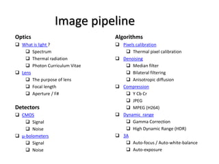
Image pipeline
Algorithms
 Pixels calibration
 Thermal pixel calibration
 Denoising
 Median filter
 Bilateral filtering
 Anisotropic diffusion
 Compression
 Y Cb Cr
 JPEG
 MPEG (H264)
 Dynamic range
 Gamma Correction
 High Dynamic Range (HDR)
 3A
 Auto-focus / Auto-white-balance
 Auto-exposure
Optics
 What is light ?
 Spectrum
 Thermal radiation
 Photon Curriculum Vitae
 Lens
 The purpose of lens
 Focal length
 Aperture / F#
Detectors
 CMOS
 Signal
 Noise
 μ-bolometers
 Signal
 Noise

‫האור‬ ‫מהות‬
‫פיזיקלית‬ ‫תורה‬‫תוקף‬ ‫פגות‬‫נשא‬‫תופעה‬‫לדוגמה‬
‫קוונטית‬ ‫פיזיקה‬‫תקף‬ ‫תמיד‬‫פוטונים‬‫לייזרים‬
‫קרינת‬‫שחור‬ ‫גוף‬
‫משוואות‬‫מקסוול‬‫אנרגיה‬<hν‫חשמלי‬ ‫שדה‬)‫ומגנטי‬)‫ה‬ ‫צבע‬‫שמיים‬
‫הגלים‬ ‫תורת‬‫הגל‬ ‫למקור‬ ‫קרוב‬‫אלקטרומגנטיים‬ ‫גלים‬‫אנטי‬ ‫ציפוי‬-‫רפלקטיבי‬
‫מצפל‬‫אלומה‬‫דיכרואי‬
‫גיאומטרית‬ ‫אופטיקה‬‫מימד‬‫פיזי‬≤‫גל‬ ‫אורך‬‫אור‬ ‫קרני‬‫אברציות‬
‫פרקסיאלית‬ ‫אופטיקה‬Sin(θ) < θ‫קרניים‬‫פרקסיאליות‬‫הגדלה‬‫אופטית‬

‫האור‬ ‫של‬ ‫הפיזיקליים‬ ‫המודלים‬ ‫שקילות‬
‫השני‬ ‫כחוט‬ ‫עובר‬ ‫פרמה‬ ‫עקרון‬
‫הפיזיקליים‬ ‫המודלים‬ ‫כל‬ ‫בין‬

Spectrum
‫האור‬ ‫מהירות‬=‫גל‬ ‫אורך‬ X‫תדר‬
‫קשת‬ ‫נוצרת‬ ‫איך‬?
‫כחולים‬ ‫השמיים‬ ‫למה‬?
‫נראה‬ ‫באור‬ ‫קורנת‬ ‫השמש‬ ‫למה‬?
‫קורן‬ ‫האדם‬ ‫גוף‬ ‫האם‬?

‫פוטון‬ ‫של‬ ‫חיים‬ ‫קורות‬
•‫יצירה‬(‫שמש‬/‫להט‬ ‫מנורת‬/‫פלורוסנט‬/LED)
•‫לצבע‬ ‫כמקור‬ ‫בליעה‬
•‫פיזור‬‫ספקולרי‬/‫דיפוזיבי‬
•‫לאישון‬ ‫המגיע‬ ‫האור‬ ‫עוצמת‬
•‫העין‬ ‫ברשתית‬ ‫בליעה‬

Algorithms
 Denoising
 Compression
 Y Cb Cr
 JPEG
 MPEG (H264)
 Dynamic range
 3A
 Auto-white-balance
 Auto-focus
 Auto-exposure
Optics
 What is light ?
 Spectrum
 Visible Light Curriculum Vitae
Lens
 Focal length
 Numerical Aperture / F#
Detectors
 CMOS
 Signal
 Noise
 μ-bolometers
 Signal
 Noise
Image pipeline

‫מוקד‬ ‫אורך‬
‫אורך‬‫מוקד‬  ‫הדמות‬ ‫מיקום‬ ‫הגלאי‬ ‫מיקום‬ 
‫ראייה‬ ‫שדה‬‫האופטי‬ ‫התכן‬ ‫מורכבות‬

‫העדשה‬ ‫מפתח‬
‫השפעות‬: ‫מורכבות‬‫התכן‬‫האופטי‬
‫עומק‬‫השדה‬ ‫כמות‬‫האנרגיה‬‫פר‬‫פיקסל‬
‫הגדרה‬:F# = f/D

Algorithms
 Denoising
 Compression
 Y Cb Cr
 JPEG
 MPEG (H264)
 Dynamic range
 3A
 Auto-focus
 Auto-exposure
Optics
 What is light ?
 Spectrum
 Lens
 Focal length
Detectors
CMOS
 Signal
 Noise
 μ-bolometers
 Signal
 Noise
Image pipeline

‫פוטודיודה‬–‫לחשמלי‬ ‫אופטי‬ ‫סיגנל‬ ‫המרת‬
N-type-Silicon
- - - - - - - - - - - -
- - - - - - - - - - - -
- - - - - - - - - - - -
- - - - - - - - - - - -
P-type-Silicon
+ + + + + + + + + + + +
+ + + + + + + + + + + +
+ + + + + + + + + + + +
+ + + + + + + + + + + +
+
-
diffusion
-
+
electrical fieldE0 0 0 0 0 0 0 0 0 0 0 0
+
-
h
-
+
-
-
-
+
depletion zone

Signal
• Optical Filters
– Bayer (for Color image)
– AR Coating
• Quantum Efficiency
–Fill factor / Micro lens / Back illumination
• Integration time and size
• Analog to Digital Conversion (ADC)

ADC - Analog to Digital Converter
• Sensor converts the
continuous light signal to a
continuous electrical signal
• The analog signal is
converted to a digital signal
– at least 10 bits (even on cell
phones), often 12 or more
– (roughly) linear sensor
response

ISO = amplification in AD conversion
Before conversion the signal can be amplified
ISO 100 means no amplification
ISO 1600 means 16x amplification
 can see details in dark areas better
 noise is amplified as well; sensor more likely to saturate

Interpolation
Fails at sharp edges
More sophisticated filterBilinear interpolation
Estimate: G @ +
Based on: G @ ·

Zippering artifact
In this area R = G = B = 1
In this area R = G = B = 0
Red Pixel Value =
( – 1 – 1 + 4 – 1 + ½ + 5 + ½ = 7 ) / 8
Red Pixel Value =
( 5.5 = - 3/2*3 + 2*2 + 6 ) / 8
≠
Let’s interpolate the RED value in the above GREEN and BLUE subpixels

Noise
Noise sources
• Shot noise (quantum)
• Johnson–Nyquist noise (Thermal)
• Grid (50 Hz)
• EMC (Electro Magnetic Compatibility)
• Dark current (Exponential temperature dependence)
• Pixel non uniformity
– PRNU (Photo-Response Non-Uniformity)
– DSNU )Dark + Bias Signal Non-Uniformity )

Algorithms
 Denoising
 Compression
 Y Cb Cr
 JPEG
 MPEG (H264)
 Dynamic range
 3A
 Auto-focus
 Auto-exposure
Optics
 What is light ?
 Spectrum
 Lens
 Focal length
Detectors
 CMOS
 Signal
 Noise
 μ-bolometers
 Signal
 Noise
Image pipeline

μ-bolometers noise
• Distance (atmospheric attenuation & image size)
• Housing Temperature (affected also by wind)
• Pixels Non-Uniformity (Necessitates calibration)
FOV < 20% of
Hemisphere

Algorithms
Thermal pixel calibration
 Denoising
 Compression
 Y Cb Cr
 JPEG
 MPEG (H264)
 Dynamic range
 3A
 Auto-focus
 Auto-exposure
Optics
 What is light ?
 Spectrum
 Lens
 Focal length
Detectors
 CMOS
 Signal
 Noise
 μ-bolometers
 Signal
 Noise
Image pipeline

From “raw-raw” to RAW
• Pixel Non-Uniformity
– each pixel has a slightly different sensitivity to light
• for CMOS: ~ 1%
• for μ-bolometers: ~10% gain, ~100% offset
– reduce by calibrating an image with a flat-field image
• also mitigates the effects of vignetting
• Stuck pixels
– some pixels are turned always on or off
– identify, replace with filtered values (nearest neighbor or median)
• Dark floor (for CMOS) detectors
– Heat generates free electrons according to Boltzmann distribution
– Subtract the signal of covered pixels located around the exposed sensor

One Point NUC ?
Why offset is needed?
Why not simply subtract the shutter image ?

Why offset is needed?
Why not simply subtract the shutter image ?
One Point NUC
𝑈 𝑂𝑏𝑗𝑒𝑐𝑡 𝜗 𝐶 = 𝑈 𝑂𝑝𝑒𝑛 𝜗 𝐶 −
Ω 𝐶
𝜋
𝑈𝑠ℎ 𝜗 𝐶 ≠ 𝑈 𝑂𝑝𝑒𝑛 𝜗 𝐶 − 𝑈𝑠ℎ 𝜗 𝐶 = 𝑈 𝑂𝑏𝑗𝑒𝑐𝑡 − 𝜔 𝐹𝑂𝑉 𝑈𝑠ℎ 𝜗 𝐶
Left hand side is independent of Right hand side depends on
the camera case temperature
X

Non-Radiometric measures ΔT (Temperature difference)
Radiometric measures T (Object Temperature)
but necessitates more calibrations

Denoising
• Median is better than average
• Bilateral filtering
• Anisotropic diffusion
• Non-local means

2D Median Filtering
Original Image
Filtered Image
Filtered Image
Filter
Filter

Eg. Median Filter – Impulsive Noise

Department of Computer Science and Engineering, Hanyang University
Spatial LPF, BPF, HPF
Spatial
averaging
),( nmu ),( nmVLP
LPF
+
),( nmVHP
),( nmu
LPF
LPF
),(1
nmhL
),(2
nmhL
+
),( nmVBP),( nmu
(a) Spatial low-pass filter (b) Spatial high-pass filter
(c) Spatial band-pass filter
),(),(),(
),(),(),(
21
nmhnmhnmh
nmhnmnmh
LLBP
LPHP

 

Denoising by Low Pass Filter
(LPF could be e.g. local average)
Noisy! Blurred! Trade-off?

Directional Smoothing
 Directional Smoothing
 to protect the edges from blurring while smoothing
):,(),(
),(
1
):,(
),(



 



nmvnmv
lnkmy
N
nmv
lk W
|):,(),(|min 

 

nmvnmythatsuch
outFind




 
W
l
k
  directionseveralincalculatedare,,averagesspatial nmv

Original image Lowpass Filter(Long Term)
Direc. Smoothing (대각선) Direc. Smoothing (수 직)
Eg. Directional Smoothing

Bilateral filter
A bilateral filter is a non-linear, edge-preserving, and noise-reducing smoothing filter for images.

The bilateral filter in its direct form can introduce several types of image artifacts:
• Staircase effect – intensity plateaus that lead to images appearing like cartoons[3]
• Gradient reversal – introduction of false edges in the image.[4]

inhomogeneous and nonlinear or Perona-Malik diffusion
http://bioen.utah.edu/wiki/images/d/d8/peronamalik90.pdf cited by 13541 articles !

Anisotropic approach
main drawback of the non-linear approach we saw earlier,
was lack of intra-edge smoothing
Solution: shape-adapted smoothing

Original
Linear isotropic diffusion
(simple gaussian)

Original
Non-linear isotropic
diffusion (edge skipping)

Original Non-linear anisotropic diffusion

Denoising using non-local means
• Most image details occur
repeatedly
• Each color indicates a group
of squares in the image
which are almost
indistinguishable
• Image self-similarity can be
used to eliminate noise
– it suffices to average the
squares which resemble
each other

4
Y Cb Cr
ITU-R BT.601 defines Y′CbCr in terms of R'G'B' as follows:
The prime ′ symbols mean gamma correction is being used;
thus R′, G′ and B′ nominally range from 0 to 1
Y “Luma” (Brightness) can be stored and transmitted with high resolution
CB , CR Chroma (Color) can be subsampled or compressed
The subsampling scheme is commonly expressed as a three part ratio J:a:b (e.g. 4:2:0)
Y = 1/4 R + 5/8 G + 1/8 B works fine and quicker to compute: R>>2 + G>>1 + G>>3 + B>>3

Further compression - JPEG Coding
Y
Cb
Cr
DPCM
RLC
Entropy
Coding
Header
Tables
Data
Coding
Tables
Quant…
Tables
DCT
f(i, j)
8 x 8
F(u, v)
8 x 8
Quantization
Fq(u, v)
Zig Zag
Scan
Steps Involved:
1. Discrete Cosine
Transform of each 8x8
pixel array
f(x,y) T F(u,v)
2. Quantization using a
table or using a constant
3. Zig-Zag scan to exploit
redundancy
4. Differential Pulse Code
Modulation(DPCM) on
the DC component and
Run length Coding of the
AC components
5. Entropy coding
(Huffman) of the final
output
More details are provided in the appendix
at the end of this presentation

Even further compression – H264
• A frame of video is one screenshot.
• Code frames as two types
– I-frames or Intra-coded frames: Coded by exploiting redundancy within
the frame
• You can think of these as being just the JPEG coding of the frame
• These are reference points in the video sequence
– P-frames or Inter-coded frames
• These are codings of frames that exploit their similarity with previously coded
frames
• Also called predicted or pseudo frames
• An example Frame Sequence:
J
P
E
G
I P P P P PI
J
P
E
G
I
J
P
E
G
MPEG-4 is a digital media compression standard
while H.264 is a component of the standard specifying digital video compression.

Appendix - JPEG Details
Multimedia Systems (Module 4 Lesson 1)
Summary:
• JPEG Compression
– DCT
– Quantization
– Zig-Zag Scan
– RLE and DPCM
– Entropy Coding
• JPEG Modes
– Sequential
– Lossless
– Progressive
– Hierarchical

Why JPEG
• The compression ratio of lossless methods (e.g., Huffman,
Arithmetic, LZW) is not high enough for image and video
compression.
• JPEG uses transform coding, it is largely based on the
following observations:
– Observation 1: A large majority of useful image contents change
relatively slowly across images, i.e., it is unusual for intensity
values to alter up and down several times in a small area, for
example, within an 8 x 8 image block.
A translation of this fact into the spatial frequency domain,
implies, generally, lower spatial frequency components contain
more information than the high frequency components which
often correspond to less useful details and noises.
– Observation 2: Experiments suggest that humans are more
immune to loss of higher spatial frequency components than loss
of lower frequency components.

JPEG Coding
Y
Cb
Cr
DPCM
RLC
Entropy
Coding
Header
Tables
Data
Coding
Tables
Quant…
Tables
DCT
f(i, j)
8 x 8
F(u, v)
8 x 8
Quantization
Fq(u, v)
Zig Zag
Scan
Steps Involved:
1. Discrete Cosine
Transform of each 8x8
pixel array
f(x,y) T F(u,v)
2. Quantization using a
table or using a constant
3. Zig-Zag scan to exploit
redundancy
4. Differential Pulse Code
Modulation(DPCM) on
the DC component and
Run length Coding of the
AC components
5. Entropy coding
(Huffman) of the final
output

DCT : Discrete Cosine Transform
DCT converts the information contained in a block(8x8) of pixels from
spatial domain to the frequency domain.
– A simple analogy: Consider a unsorted list of 12 numbers between 0 and
3 -> (2, 3, 1, 2, 2, 0, 1, 1, 0, 1, 0, 0). Consider a transformation of the list
involving two steps (1.) sort the list (2.) Count the frequency of
occurrence of each of the numbers ->(4,4,3,1 ). : Through this
transformation we lost the spatial information but captured the
frequency information.
– There are other transformations which retain the spatial information.
E.g., Fourier transform, DCT etc. Therefore allowing us to move back and
forth between spatial and frequency domains.
1-D DCT: 1-D Inverese DCT:

F() a(u)
2
f(n)cos
(2n1)
16
n  0
N1

a(0) 1
2
a(p)1 p0 

f'(n) a(u)
2
F()cos
(2n1)
16
  0
N1


Example and Comparison
0
20
40
60
80
0 1 2 3 4 5 6 7
100 -52 0 -5 0 -2 0 0.4 36 10 10 6 6 4 4 4
36 10 10 6 6 4 4 4100 -52 0 -5 0 -2 0 0.4
24 12 20 32 40 51 59 488 15 24 32 40 48 57 63
0
20
40
60
80
0 1 2 3 4 5 6 7
0
20
40
60
80
0 1 2 3 4 5 6 7
DCT FFT
Inverse DCT Inverse FFT
Example Description:
r f(n) is given from n = 0 to 7; (N=8)
r Using DCT(FFT) we compute F(ω) for ω = 0 to 7
r We truncate and use Inverse Transform to compute f’(n)

2-D DCT
• Images are two-dimensional; How do you perform 2-D DCT?
– Two series of 1-D transforms result in a 2-D transform as demonstrated in
the figure below
1-D
Row-
wise
1-D
Column-
wise
8x8 8x8 8x8
j)f(i,
v)F(u,
r F(0,0) is called the DC component and the rest of F(i,j) are called
AC components

2-D Transform Example
• The following example will demonstrate the idea behind a 2-D
transform by using our own cooked up transform: The transform
computes a running cumulative sum.
1
1-D
Row-
wise
1-D
Column-
wise
8x8
8x8
8x8
1
1
1
1
1
1
1
1
1
1
1
1
1
1
1
1
1
1
1
1
1
1
1
1
1
1
1
1
1
1
1
1
1
1
1
1
1
1
1
1
1
1
1
1
1
1
1
1
1
1
1
1
1
1
1
1
1
1
1
1
1
1
1
8 7 6 5 4 3 2 1
8 7 6 5 4 3 2 1
8 7 6 5 4 3 2 1
8 7 6 5 4 3 2 1
8 7 6 5 4 3 2 1
8 7 6 5 4 3 2 1
8 7 6 5 4 3 2 1
8 7 6 5 4 3 2 1
64 56 48 40 32 24 16 8
56
48
40
32
24
16
8
49
42
35
28
21
14
7
42
36
30
24
18
12
6
35
30
25
20
15
10
5
28
24
20
16
12
8
4
21
18
15
12
9
6
3
14
12
10
8
6
4
2
7
6
5
4
3
2
1
 

8
nmy (n)f)(F 
My Transform:
j)f(i,
v)(u,myF
Note that this is only a hypothetical
transform. Do not confuse this with DCT

Quantization
• Why? -- To reduce number of bits per sample
F’(u,v) = round(F(u,v)/q(u,v))
• Example: 101101 = 45 (6 bits).
Truncate to 4 bits: 1011 = 11. (Compare 11 x 4 =44 against 45)
Truncate to 3 bits: 101 = 5. (Compare 8 x 5 =40 against 45)
Note, that the more bits we truncate the more precision we lose
• Quantization error is the main source of the Lossy Compression.
• Uniform Quantization:
– q(u,v) is a constant.
• Non-uniform Quantization -- Quantization Tables
– Eye is most sensitive to low frequencies (upper left corner in frequency
matrix), less sensitive to high frequencies (lower right corner)
– Custom quantization tables can be put in image/scan header.
– JPEG Standard defines two default quantization tables, one each for
luminance and chrominance.

Zig-Zag Scan
• Why? -- to group low frequency coefficients in top of vector and high
frequency coefficients at the bottom
• Maps 8 x 8 matrix to a 1 x 64 vector
8x8
. . .
1x64

DPCM on DC Components
• The DC component value in each 8x8 block is large and varies across
blocks, but is often close to that in the previous block.
• Differential Pulse Code Modulation (DPCM): Encode the difference
between the current and previous 8x8 block. Remember, smaller
number -> fewer bits
45
54
48
32
45
9
-6
12
36 4
.
.
.
.
.
.
1x64
1x64
1x64
1x64
1x64
1x64
1x64
1x64
1x64
1x64

RLE on AC Components
• The 1x64 vectors have a lot of zeros in them, more so towards the end
of the vector.
– Higher up entries in the vector capture higher frequency (DCT) components
which tend to be capture less of the content.
– Could have been as a result of using a quantization table
• Encode a series of 0s as a (skip,value) pair, where skip is the number of
zeros and value is the next non-zero component.
– Send (0,0) as end-of-block sentinel value.
. . .
1x64
0 0 0 0 0 1 1 0 0 0 0 0
5,1
0 0
7,2
0 . . .2

Entropy Coding: DC Components
• DC components are differentially coded as (SIZE,Value)
– The code for a Value is derived from the following table
SIZE Value Code
0 0 ---
1 -1,1 0,1
2 -3, -2, 2,3 00,01,10,11
3 -7,…, -4, 4,…, 7 000,…, 011, 100,…111
4 -15,…, -8, 8,…, 15 0000,…, 0111, 1000,…, 1111
. .
. .
11 -2047,…, -1024, 1024,… 2047 …
Size_and_Value Table

How many bits are needed for smooth shading?
• human vision has contrast sensitivity ~1%
• call black 1, white 100
• you can see differences between:
• 1, 1.01, 1.02, … needed step size ~ 0.01
• 98, 99, 100 needed step size ~ 1
• with linear encoding
• delta 0.01
– 100 steps between 99 & 100  wasteful
• delta 1
– only 1 step between 1 & 2  lose detail in shadows
• instead, apply a non-linear power function, gamma
• provides adaptive step size
• 8 bits span contrast ratio of 13:1
• 1.01^(2^8) ≈ 13
• More accurately: 1%  1.5%,
13  1.015^(2^8) ≈ 45

Gamma Correction
compress
stretch
1 < γ0 < γ < 1
𝑔 =
𝑓 𝛾
[𝑅𝑎𝑛𝑔𝑒 𝑓] 𝛾
~𝑓 𝛾

Concatenated Gamma (γ)
γdisplay
Signalout ~ Signalin ^ γ  γtotal = γdetector x γImageEnhancement x γdisplay
Image processing better be implemented in linear space, γ = 1/ γdetector

High Dynamic Range HDR
•‫שצג‬ ‫ראינו‬ ‫קודם‬8‫של‬ ‫קונטרסט‬ ‫מאפשר‬ ‫ביט‬45:1‫רזולוציה‬ ‫אובדן‬ ‫ללא‬,
‫במתיחת‬ ‫שימוש‬ ‫תוך‬:γ1.015^(2^8) ≈ 45
•‫מתיחת‬ ‫אין‬ ‫בגלאי‬γ,‫קונטרסט‬ ‫לאותו‬ ‫להגיע‬ ‫כדי‬ ‫לכן‬,‫נדרשים‬12‫ביטים‬
1.015*(2^12) ≈ 1.015^(2^8)
•‫מספיק‬ ‫לא‬ ‫זה‬ ‫גם‬ ‫אבל‬
‫יותר‬ ‫הרבה‬ ‫גדול‬ ‫טיפוסית‬ ‫בתמונה‬ ‫הקונטרסט‬ ‫כי‬
•‫חשיפות‬ ‫מספר‬ ‫ידי‬ ‫על‬ ‫הגלאי‬ ‫של‬ ‫הדינמי‬ ‫התחום‬ ‫את‬ ‫להגדיל‬ ‫אפשר‬
(automatic exposure bracketing)‫פריים‬ ‫בכל‬

A ‘bit’ of conversion
12-bit
RAW
12-bit
RAW
12-bit
RAW
8-bit
32-bit HDR
8-bit
HDR8-bit
8-bit
RAW Conversion
(optional)
Exposure Blending
Tone Mapping
(Dynamic Range
Compression)

Simple contrast reduction
Local tone mapping
Every pixel in the image is mapped in the same way, independent of the value of surrounding
pixels in the image, according to a global function e.g. from 32 bits to 12 bits.
Gamma Correction is an examples of global tone mapping
Histogram Equalization is another more effective example
Those techniques are simple and fast, but they can cause a loss of contrast.

TMO (Tone Mapping Operations) methods
• https://www.cl.cam.ac.uk/~rkm38/pdfs/tone_mapping.pdf
• https://www.cl.cam.ac.uk/~rkm38/pdfs/eilertsen2017tmo_star.pdf
• https://www.cl.cam.ac.uk/~rkm38/pdfs/mantiuk15hdri.pdf
• https://www.cl.cam.ac.uk/~rkm38/pdfs/myszkowski08hdrvideo.pdf

Auto-white-balance
• The dominant light source (illuminant) produces a color
cast that affects the appearance of the scene objects
• The color of the illuminant determines the color
normally associated with white by the human visual
system
• Auto-white-balance
– Identify the illuminant color
– Neutralize the color of the illuminant

Contrast-based auto-focus
• ISP can filter pixels with configurable IIR filters
– to produce a low-resolution sharpness map of the image
• The sharpness map helps estimate the best lens
position
– by summing the sharpness values
• either over the entire image
• or over a rectangular area
Phase Detect
auto-focus

Auto-exposure
• Goal: well-exposed image
Possible parameters to adjust:
– Exposure time
• Longer exposure leads to brighter image and better SNR
• but also motion blur and saturation
– Aperture (f-number)
• Smaller F# also leads to brighter image and better SNR
• but also decreased Depth of focus and saturation
– Analog and digital gain
• Higher gain makes image brighter but amplifies noise as well

Exposure metering
May be applied to either the full frame or central region of interest

Image Enhancement
Histogram Manipulations
Stretching (J3)
Equalization
CLAHE
FLIR’s histogram equalization
Plateau Equalization (Day and Night)
Information-Based Equalization
Low light (L6)
Invert - de-haze – Revert (L6)

Image Histograms
• An image histogram is a plot of the gray-level frequencies (i.e.,
the number of pixels in the image that have that gray level).

Sometimes histogram stretching
is better than histogram equalization

And sometimes histogram stretching
is useless

Image Histograms (cont’d)
• Divide frequencies by total number of pixels to represent
as probabilities.
Nnp kk /=

Histogram Equalization (cont’d)
de-normalize:
sk x (L-1)
𝑟𝑖+1 > 𝑟𝑖 ∀𝑖
𝑃𝑆 𝑠𝑗 =
𝑘
𝑗=0
𝑃𝑟 𝑟𝑗
𝑘
𝑗=0
= 𝑠 𝑘
Why does the T transformation
generates equalized histogram ?
𝑃 𝑠 𝑑𝑠
𝑠 𝑘
0
= 𝑠 𝑘 𝑖𝑓𝑓
𝑃 𝑠 =
1 𝑓𝑜𝑟 0 < 𝑠 < 1
0 𝑒𝑙𝑠𝑒

Explicit Algorithm for Histogram equalization
For an M * N image of G gray-levels, create two arrays H and T of length G
initialized with 0 values. Form the image histogram: scan every pixel and
increment the relevant member of H. If pixel X has intensity p, perform:
Form the cumulative image histogram Hc and store the result in the same array H
Rescan the image and write an output image with gray-levels q by setting
Copied from: AN EFFICIENT VIDEO ENHANCEMENT METHOD USING LA*B* ANALYSIS
Gaurav Mittal, Sushrutha Locharam & Sreela Sasi Glenn R. Shaffer & Ajith K. Kumar

AHE - Adaptive Histogram Equalization
For each pixel
Use only the pixels in its neighborhood
in order to calculate the transformation

CLAHE Contrast Limited AHE
CLAHE was developed to prevent
the over amplification of noise
that AHE may introduce.
CLAHE limits the amplification by
clipping the histogram at a predefined
value before computing the CDF.

Plateau Equalization
(used by FLIR in most products)
In classical Histogram equalization:
𝑠 𝑘 =
𝑁𝑖
𝑘
𝑗=0
𝑛
In practice, for 14 bit data, binning should be implemented, e.g. to 8 bit bins:
𝑁𝑖 = 𝑛𝑗
26∗ 𝑖+1 −1
𝑗=2(14−8)∗𝑖
, 𝑖 ∈ (0,255)
So the binning changes the classical histogram equalization to:
In ‘Plateau Equalization’ the bins values are modified as follows:
•
•
𝑁𝑖 = min( 𝑁𝑖 , const ~ "Linear Percent" ) to ensure grayscale separation between different temperatures
𝑁𝑖 = max( 𝑁𝑖 , "Plateau Value" ∗ n ) In order not to waste too many gray levels on uniform regions (like the sky)
𝑠 𝑘 =
𝑁𝑖
𝑘
𝑗=0
𝑁𝑖
255
𝑗=0
Thus in Plateau Equalization the transformation is:

Plateau Equalization
Additional parameters
There are few more parameters that define FLIR’s transformation,
but those values are more general to video histogram manipulation
(not specific to thermal data)

Information-Based Equalization
(used in Boson enabled by Movidius)
The scene data is segregated into details and
background using a High-Pass (HP) and Low-Pass
(LP) filter. Pixel values in the HP image are weighted
more heavily during the histogram-generation.

Low light image enhancement
According to “A Survey of Video Enhancement
Techniques” by Yunbo Rao, Leiting Chen (2011)
Only two methods are applicable to real time
low light videos:
1. Apply Histrogram Equalization to the Y
channel in Y Cb Cr
2. Invert – de-haze – Revert, as will be
elaborated in the next slides
1. AN EFFICIENT VIDEO ENHANCEMENT METHOD USING LA*B* ANALYSIS
Gaurav Mittal, Sushrutha Locharam & Sreela Sasi Glenn R. Shaffer & Ajith K. Kumar
2. Fast efficient algorithm for enhancement of low lighting video
X. Dong, Y. Pang and J.Wen, (2010)

Let’s dwell into the inspiring algorithm:
Dehaze
Mathematical Model of Atmospheric Scattering :
• I(x) is the observed radiance at x
• J(x) is the original scene radiance at x
• A is the airlight
• t(x), scalar called transmission: describes how the radiance of a point in the
scene is attenuated according to its distance d from the observer
• Note that I, J, A are (R,G,B) triplets

The Atmospheric Scattering Model
Mathematical Model:
• In order to remove the effect of haze, one must recover J(x)
• Quantities A and t are typically unknown
• I(x) is known

• In every region there is a ”dark channel” for which the object has
negligible contribution to the signal.
• Out of the intensities that correspond to the Jdark(x)
the top percentile stems from long distanced objects (or the sky)
• Thus the average intensity of the brightest dark channel
estimates the airlight = A
“Single Image Haze Removal Using Dark Channel Prior”
A (airlight) estimation
𝐵𝑟𝑖𝑔ℎ𝑡𝑒𝑠𝑡 𝑑𝑎𝑟𝑘 𝑐ℎ𝑎𝑛𝑛𝑒𝑙
0
𝐵𝑟𝑖𝑔ℎ𝑡𝑒𝑠𝑡 𝑑𝑎𝑟𝑘 𝑐ℎ𝑎𝑛𝑛𝑒𝑙
A
≈0

“Single Image Haze Removal Using Dark Channel Prior”
transmission t(x) estimation
Since the observed intensity corresponding to the dark channel stems
only from the airlight (for both far and close objects).
The transmission (and hence also the distance)
can be estimated by calculating:
Dark channel of the region
divided by the airlight color
And the Recovery equation is:
𝐽 𝑥 =
𝐼 𝑥 − 𝐴 1 − 𝑡 𝑥
𝑡 𝑥
=
𝐼 𝑥 − 𝐴
𝑡 𝑥
+ 𝐴

“FAST EFFICIENT ALGORITHM FOR ENHANCEMENT OF LOW LIGHTING VIDEO”
𝐽 𝑥 =
𝐼 𝑥 − 𝐴
P(x) 𝑡 𝑥
+ 𝐴
The above mentioned ‘equation (7)’ is a just a minor modification of the Recovery equation
from previous slide:
With the modification being:‫המאמר‬ ‫תקציר‬
‫ניתן‬‫להורדה‬
‫זה‬ ‫בקישור‬

Edge detection
Convert a 2D image into a set of curves
• Extracts salient features of the scene
• More compact than pixels

The discrete gradient
How can we differentiate a digital image f[x,y]?
• Option 1: reconstruct a continuous image, then take gradient
• Option 2: take discrete derivative (finite difference)
How would you implement this as a cross-correlation?

The Sobel operator
Better approximations of the derivatives exist
• The Sobel operators below are very commonly used
-1 0 1
-2 0 2
-1 0 1
1 2 1
0 0 0
-1 -2 -1
• The standard defn. of the Sobel operator omits the 1/8 term
– doesn’t make a difference for edge detection
– the 1/8 term is needed to get the right gradient value, however

Effects of noise
Consider a single row or column of the image
• Plotting intensity as a function of position gives a signal
Where is the edge?

Where is the edge?
Solution: smooth first
Look for peaks in

Derivative theorem of convolution
This saves us one operation:

Laplacian of Gaussian
Consider
operator
Where is the edge? Zero-crossings of bottom graph

2D edge detection filters
is the Laplacian operator:
Gaussian derivative of Gaussian

The Canny edge detector
original image (Lena)

norm of the gradient

thresholding

Non-maximum suppression
Check if pixel is local maximum along gradient direction
• requires checking interpolated pixels p and r

thinning
(non-maximum suppression)
& Hysteresys

Hysteresis
Check that maximum value of gradient value is
sufficiently large
• drop-outs? use hysteresis
– use a high threshold to start edge curves and a low threshold to
continue them.

The challenges of edge detection
Texture
Low-contrast boundaries

Fusion
• Registration
• Pixel-Based Opponent-Color Fusion
• Gaussian & Laplacian pyramids
• Fused pictures from Nyx – 211 and public domain
• Other methods (Literature Review)

Pixel-Based Opponent-Color Fusion
‫מתוך‬ ‫המקורי‬ ‫האלגוריתם‬‫המאמר‬Progress in color night vision:
‫מבין‬ ‫פיקסל‬ ‫כל‬ ‫עבור‬VGA‫פיקסלים‬,
‫בצג‬ ‫הפיקסל‬ ‫ערכי‬(R, G, B)‫של‬ ‫הפיקסל‬ ‫בערך‬ ‫תלויים‬‫הסיוניקס‬(I_Sionyx)‫התרמי‬ ‫ושל‬
(I_Therm)‫כלהלן‬:
• MIN = Min { I_Sionyx , I_Therm }
• I_Sionyx* = I_Sionyx – MIN
• I_Therm* = I_Therm – MIN
• R = I_Therm - I_Sionyx*
• G = I_Sionyx - I_Therm*
• B = I_Therm* - I_Sionyx*
‫שיושם‬ ‫האלגוריתם‬:
•‫טריוויאלי‬ ‫הכי‬ ‫באופן‬ ‫הדינמי‬ ‫התחום‬ ‫מתיחת‬:
I_new = (I_old - I_GlobalMin) / (_GlobalMax - I_GlobalMin)
•‫המקורי‬ ‫האלגוריתם‬ ‫יישום‬
•‫הכחול‬ ‫בערוץ‬ ‫הסיגנל‬ ‫הנמכת‬:G  G / 2

2)*( 23  gaussianGG
1G
The Gaussian Pyramid
High resolution
Low resolution
Image0G
blur
blur
blur
blur

Gaussian Pyramid Laplacian Pyramid
The Laplacian Pyramid
0G
1G
2G
nG
- =
0L
- =
1L
- = 2L
nn GL 
)expand( 1 iii GGL
)expand( 1 iii GLG

Gaussian Pyramid Laplacian Pyramid
The Laplacian Pyramid
0G
1G
2G
nG
= +
0L
= +
1L
= + 2L
nn GL 
)expand( 1 iii GGL
)expand( 1 iii GLG

Image Fusion
Multi-scale Transform (MST) = Obtain Pyramid from Image
Inverse Multi-scale Transform (IMST) = Obtain Image from Pyramid

IR in Red ; VIS in Green as Captured from U211 (without any image processing or registration)

Pixel-Based Opponent-Color Fusion

LP fusion without registration

A survey of infrared and visual image fusion methods
from Infrared Physics & Technology (2017)
24 pages with Kwords per page and 177 References
Summarized to 1 slide:
IR + VIS algorithms
Feature (edges and textures)
e.g. bilateral filter
Signal (Pixels)
Minimum artifacts in the fused image
Spatial domain
e.g. IR in Red, Vis in Green
and Gradient transfer
Transform domain
e.g Laplacian pyramids, Wavelet,
symbol (Humans)
e.g. Sparse Rep.
Generally, traditional algorithms cannot be used for video fusion
due to the limitation of timeliness 
Specifically, Non-subsampled transform performs the best, “however, the high computational
complexity limits the application in real-time applications”

Infrared and visible image fusion methods
and applications: A survey (2018)
with 325 references
The experiments are conducted on a desktop
with 3.3 GHz Intel Core CPU, 8 GB memory, and MATLAB codes.
Real time implementation use: FPGA or CUDA (Not DSP)

Infrared and …. A survey (2018) Results

Range finding
 Stereoscopic
 Structured light (Kinect etc.)
 Time of flight (LRF)
 CW range finder (Innovative idea)
 Auto focus phase detector (used by Aptina / On semiconductors)

Introduction to
Computer Vision Disparity and Depth
 If the cameras are pointing in
the same direction, the
geometry is simple.
 b is the baseline of the camera
system,
 Z is the depth of the object,
 d is the disparity (left x minus
right x) and
 f is the focal length of the
cameras.
 Then the unknown depth is
given by
b
Z =
f b
d

Introduction to
Computer Vision Converging Cameras
 This is the more realistic case.
 The depth at which the cameras
converge, Z0, is the depth at
which objects have zero disparity.
 Finding Z0 is part of stereo
calibration.
 Closer objects have convergent
disparity (numerically positive)
and further objects have divergent
disparity (numerically negative).
Object at
depth Z

Lagrange Multipliers
Maximize f(x,y)
f in RWS: the difference between:
{ LEDs locations (x,y) } to { the measured locations (x*, y*) }
Subject to g(x,y)
g in RWS: the difference between:
{ the LEDs distance ( x-y ) } to the
{ predefined distance during assembly }
The Lagrange multipliers method for Solution:

Introduction to Computer Vision
• Extraction of edges
• Representation of objects as interconnections of smaller structures,
• Pattern matching
• Eigen face

Computer Vision as a function
• A function is a kind of mapping
• In computer vision we seek for a function
that maps an image (a digital signal)
to a piece of information (e.g. – it is a cat)
• Since there are finite number of possible images,
a-priori it should be straightforward
• However, the number of possible images is larger than the
number of atoms in the universe

Information theory (Signal processing)
Shannon Entropy quantifies
The minimum number of bits required to deliver
the data in a signal

Classical Approach
HandCraftedFilters
Hand crafted
Filter 1
• Original Image
Hand crafted
Filter 2
• Processed Image 1
Hand crafted
Filter 3
• Processed Image 2
…
• …
Hand crafted
Filter n+1
• Processed Image n
Output
• Result

‫נוירונים‬ ‫רשתות‬ ‫של‬ ‫מההצלחה‬ ‫מסקנות‬
•‫רבוד‬ ‫מציאותיות‬ ‫בתמונות‬ ‫המידע‬
•‫המידע‬ ‫את‬ ‫לזקק‬ ‫כדי‬(‫השכבות‬ ‫את‬ ‫לקלף‬)
‫מורכבות‬ ‫בפונקציות‬ ‫להשתמש‬ ‫עדיף‬
•‫האופטימלי‬ ‫המורכבות‬ ‫עומק‬
‫ההיסק‬ ‫במערכת‬ ‫לתמוך‬ ‫האנושית‬ ‫מהקיבולת‬ ‫גבוה‬
–‫האנושית‬ ‫הקיבולת‬ ‫במסגרת‬ ‫היסק‬ ‫למערכת‬ ‫דוגמא‬:
•‫ראשונה‬ ‫שכבה‬:‫בתמונה‬ ‫פינות‬ ‫למצוא‬
•‫שנייה‬ ‫שכבה‬:‫מסוים‬ ‫יחס‬ ‫מקיימים‬ ‫הפינות‬ ‫בין‬ ‫המרחקים‬ ‫האם‬ ‫לבדוק‬
•‫שלישית‬ ‫שכבה‬:‫הקודם‬ ‫הפריים‬ ‫מאז‬ ‫הפינות‬ ‫מערכת‬ ‫מיקום‬ ‫שינוי‬ ‫חישוב‬
•‫תוצאה‬:‫האובייקט‬ ‫תנועת‬

‫נוירונים‬ ‫רשתות‬
•‫נוירונים‬ ‫רשת‬ ‫מהי‬?
•‫איך‬"‫מלמדים‬"‫הרשת‬ ‫את‬?
•CNN – Convolutional Neural Network
•‫הספק‬ ‫דלות‬ ‫נוירונים‬ ‫רשתות‬

Machine “2”
1x
2x
256x
……
……
y1
y2
y10𝑓: 𝑅256 → 𝑅10
In deep learning, the function 𝑓 is
represented by neural network
Handwriting Digit Recognition

‫נוירונים‬ ‫רשת‬ ‫של‬ ‫הארכיטקטורה‬

Output
LayerHidden Layers
Input
Layer
Neural Network
Input Output
1x
2x
Layer 1
……
Nx
……
Layer 2
……
Layer L
……
……
……
……
……
y1
y2
yM
Deep means many hidden layers
neuron

Example of Neural Network
 z
z
  z
e
z 


1
1

Sigmoid Function
1
-1
1
-2
1
-1
1
0
4
-2
0.98
0.12

1
-2
1
-1
1
0
4
-2
0.98
0.12
2
-1
-1
-2
3
-1
4
-1
0.86
0.11
0.62
0.83
0
0
-2
2
1
-1

1
-2
1
-1
1
0
0.73
0.5
2
-1
-1
-2
3
-1
4
-1
0.72
0.12
0.51
0.85
0
0
-2
2
𝑓
0
0
=
0.51
0.85
Different parameters define different function
𝑓
1
−1
=
0.62
0.83
𝑓: 𝑅2 → 𝑅2
0
0

How to set network parameters
16 x 16 = 256
1x
2x
……
256x
……
……
……
……
Ink → 1
No ink → 0
……
y1
y2
y10
0.1
0.7
0.2
y1 has the maximum value
Set the network parameters 𝜃 such that ……
Input:
y2 has the maximum valueInput:
is 1
is 2
is 0
How to let the neural
network achieve thisSoftmax
𝜃 = 𝑊1, 𝑏1, 𝑊2, 𝑏2, ⋯ 𝑊 𝐿, 𝑏 𝐿

Training Data
• Preparing training data: images and their
labels
Using the training data to find
the network parameters.
“5” “0” “4” “1”
“3”“1”“2”“9”

Backpropagation
• A network can have millions of parameters.
– Backpropagation is the way to compute the
gradients efficiently (not today)
– Ref:
http://speech.ee.ntu.edu.tw/~tlkagk/courses/ML
DS_2015_2/Lecture/DNN%20backprop.ecm.mp4/
index.html
• Many toolkits can compute the gradients automatically

What is Convolution?
Input Feature Map
.
.
.

Convolution as feature extraction
2x2
Convolution + NL Sub-sampling Convolution + NL

Color (RGB)
image
One 4x4x3 filter
(cube(
The result of a single filter
Another filter

A first layer of
filters
A second layer of
filters
An MNIST
image
A third layer of
filters
(treat this as 1176-D
vector)
A “fully connected”
layer (as before(

ILSVRC 2012: top rankers
http://www.image-net.org/challenges/LSVRC/2012/results.html
N Error-5 Algorithm Team Authors
1 0.153 Deep Conv. Neural Network Univ. of Toronto Krizhevsky et al
2 0.262 Features + Fisher Vectors +
Linear classifier
ISI Gunji et al
3 0.270 Features + FV + SVM OXFORD_VGG Simonyan et al
4 0.271 SIFT + FV + PQ + SVM XRCE/INRIA Perronin et al
5 0.300 Color desc. + SVM Univ. of
Amsterdam
van de Sande et al

Imagenet 2013: top rankers
http://www.image-net.org/challenges/LSVRC/2013/results.php
N Error-5 Algorithm Team Authors
1 0.117 Deep Convolutional Neural
Network
Clarifi Zeiler
Networks
Nat.Univ
Singapore
Min LIN
Networks
NYU Zeiler
Fergus
Networks
Andrew Howard
Networks
Overfeat
NYU
Pierre Sermanet et al

Visual Object Tracking (VOT)
‘State Of The Art’ (SOTA) 2016
Discriminative correlation filters (DCF) Rules
Frame
rate

Review: Discriminative correlation filters
𝑊⋆
= 𝑎𝑟𝑔𝑚𝑖𝑛 𝑊
||𝑊 ∗ 𝑋 − 𝑌||2
+ 𝜆||𝑊||2
Objective function: ridge regression.
X: input features
Y: ground truth gaussian label
W: correlation filter weight
𝑊 = (𝑋 𝑇
𝑋 + 𝜆𝐼)−1
𝑋 𝑇
𝑌
𝑓(𝑋) = 𝑊 ∗ 𝑋

Typical Siamese CNN
• Input: A pair of input signatures.
• Output (Target): A label, 0 for similar, 1 else.
Bromley, J., Bentz, J.W., Bottou, L., Guyon, I., LeCun,
Y., Moore, C., Säckinger, E. and Shah, R., 1993.
Signature Verification Using A "Siamese" Time Delay
Neural Network. IJPRAI, 7(4), pp.669-688.
Image Source:
Google
Share
Weights

Siamese NN for RT object tracking

Image pipeline

Recommandé

Recommandé

Contenu connexe

Tendances

Tendances (20)

Similaire à Image pipeline

Similaire à Image pipeline (20)

Dernier

Dernier (20)

Image pipeline