systemic_risk_final_version_ssrn

Simulation of Negative Feedback Effects in Financial
Systems∗
Pascal M. Caversaccio†
Patrick Cheridito‡
Meriton Ibraimi§
First Draft: August 28, 2014
This Version: August 6, 2015
Abstract
In a financial system of banks, which are linked through interbank lending, we postulate that
indirect spillover effects, such as funding liquidity dry-ups and asset fire sales, can play a crucial
role. Considering only direct effects, i.e. bank defaults, underestimates the extent of a crisis,
thereby showing the importance of indirect spillover effects. To model funding liquidity, we allow
banks to access the interbank lending market and as a second channel, to obtain liquidity from a
repo transaction. Additionally, the developed framework enables us to impose exogenous shocks
to the financial system; for instance bank defaults, asset price deteriorations, higher margins and
haircuts, and a sharp increase of the short-term interest rate. Consequently, this paper builds a
unified framework that can enrich the toolbox used by national banks and the European central
bank.
Keywords: Asset fire sales, contagion, direct spillover effects, indirect spillover effects, liquidity risk,
systemic risk.
JEL classification: D85, G01, G21.
∗
The authors thank Eric Jondeau and Stefan Pomberger for helpful comments. Financial support from the Swiss
Finance Institute (SFI), Bank Vontobel, the Swiss National Science Foundation, and the National Center of Competence
in Research ”Financial Valuation and Risk Management” is gratefully acknowledged. Any remaining errors are ours.
†
University of Zurich – Department of Banking and Finance, Chair of Financial Engineering, Plattenstrasse 22,
8032 Zurich, Switzerland. Tel: (+41)-44-634-4586; E-Mail: pascalmarco.caversaccio@uzh.ch.
‡
Princeton University – Department of Operations Research and Financial Engineering, 204 Sherrerd Hall, 08544
Princeton, New York, United States. Tel: (+1)-609-258-8281; E-Mail: dito@princeton.edu.
§
University of Zurich – Department of Banking and Finance, Chair of Financial Engineering, Plattenstrasse 22,
8032 Zurich, Switzerland. Tel: (+41)-44-634-4045; E-Mail: meriton.ibraimi@uzh.ch.

Simulation of Negative Feedback Effects in Financial
Systems
August 6, 2015
Abstract
In a financial system of banks, which are linked through interbank lending, we postulate that
indirect spillover effects, such as funding liquidity dry-ups and asset fire sales, can play a crucial
role. Considering only direct effects, i.e. bank defaults, underestimates the extent of a crisis,
thereby showing the importance of indirect spillover effects. To model funding liquidity, we allow
banks to access the interbank lending market and as a second channel, to obtain liquidity from a
repo transaction. Additionally, the developed framework enables us to impose exogenous shocks
to the financial system; for instance bank defaults, asset price deteriorations, higher margins and
haircuts, and a sharp increase of the short-term interest rate. Consequently, this paper builds a
unified framework that can enrich the toolbox used by national banks and the European central
bank.
Keywords: Asset fire sales, direct spillover effects, indirect spillover effects, contagion, liquidity risk,
systemic risk.
JEL classification: D85, G01, G21.

1 Introduction
What is systemic risk in finance? There is no consensus on the definition, but what we are talking
about is the risk of a collapse of a large part of the financial system and the impact on the real
economy.1 Following the 2007 – 2008 subprime mortgage crisis, the discussions on systemic risk
and the too big to fail problematic have flourished. These topics are of great interest to financial
regulators and have yet to be fully understood. This uncertainty entails the necessity of stress tests,
which simulate the evolvement of shocks through a financial system and gauge the stability of the
given entity.
We propose a stress test environment which encompasses an appropriate time frame of a few
weeks, e.g. two weeks, and consists of ten banks at its core which are linked through overnight
interbank lending activities. The terminology bank is employed to refer to any financial institution
like a commercial bank, a private bank, a retail bank, or another financial intermediary. The model
design can be easily extended to include more than ten banks, but considering a few number of banks
copes with our purpose. Also, with regard to the empirical fact that in the United States (US) 60%
of all US commercial bank assets are held only by the largest six banks, a model which includes the
ten largest banks already covers a large part of the banking sector.2 A similar qualitative structure
for the Swiss banking sector can be observed in Table 1. The two big Swiss banks, i.e. UBS AG and
Credit Suisse Group AG, hold together asset values which amount approximately 50% of the total
assets. This circumstance obviously motivates for an appropriate recovery and resolution planning
for these entities in conjunction with the too big to fail problematic. Furthermore, in Table 2 the
geographical and structural composition of the EU banking sector is depicted. Therefrom we can
not only deduce that the too big to fail problematic is subject to geographic constraints but also
that a possible too interconnected to fail problematic can lead to further spillover effects into smaller
countries. Hence, modeling a few number of influential banks is an eligible starting point in order to
control for their impact in the stress test environment.
1
See Adrian and Brunnermeier (2011) and Brunnermeier and Cheridito (2014) who introduce mathematical mea-
sures for systemic risk.
2
The same qualitative reasoning holds true for the European banking sector where for instance the HSBC Holdings
plc exhibits more than twice as much assets as the UBS AG in 2013.
1

[Table 1 about here.]
We assume each bank’s overnight interbank liabilities, and hence also the corresponding asset
values, to be constant, which is justified by the fact that in times of (financial) distress banks are
likely to have to roll over their overnight interbank liabilities over the short time frame we consider. In
our model, banks hold fully liquid assets, e.g. cash, and additionally are allowed to obtain liquidity
from entering a repurchase agreement (repo) transaction by using their repo assets as collateral.
The liabilities of a bank are decomposed into overnight interbank–, short-term (e.g. three month)–,
repo–, deposit–, and long-term (e.g. ten year) liabilities. The latter remains unaffected in our model
due to its long maturity and the short time frame we consider. Similarly, the assets of a bank are
decomposed into different classes, such as fully liquid–, overnight interbank–, repo–, and reverse repo
assets, and further (risky) assets, e.g. deposits, mortgage loans, corporate loans, derivatives, or fixed
assets. Repo assets, generally a subset of the collateral assets, are those assets which a bank can use
as collateral to obtain liquidity by entering a repo transaction. For simplicity’s sake we assume in our
framework that the collateral and repo assets, respectively, coincide. The conducted classification
yields overall a rich and flexible structure of nine (five) different asset (liability) classes.
Through the interbank lending linkages, the default of one bank can cause the default of further
banks, and this effect is referred to as the direct effect. To keep track of the evolvement of a shock
through the system, we model the balance sheet of each bank on a daily basis. If the top tier capital
ratio (TTCR) of a bank, which is the ratio of assets minus liabilities over risk-weighted assets,3 falls
below a certain threshold value (e.g. 7%), we say that this bank defaults. Along with the direct effect,
the so-called indirect effects can take place. These effects are, among others, increasing margins and
haircuts in the repo market, increasing interest rates on short-term (unsecured) lending, and fire
sales. At t = 1 we model the indirect effects independently of the direct effects. However, these
indirect effects are crucial drivers for recurring direct effects for t > 1. Our model allows to shock
the system in various ways, resulting in manifold triggers of a crisis. All shocks occur at time t = 1
3
We refer to Eq. (1) for the exact mathematical representation.
2

and can be, among others, an arbitrary large asset price deterioration, an immediate default of a
bank, or an arbitrary increase of aggregate and/or bank specific margins and haircuts. Moreover, by
imposing a liquidity measure we can assess a bank’s overnight liquidity at any point in time.
Our paper is based on the findings of Brunnermeier (2009) and Afonso et al. (2011). Brunnermeier
(2009) argues that fire sales were an amplifying effect to the 2007 – 2008 financial crisis. In Afonso
et al. (2011), empirical evidence is given for a funding dry-up in the interbank and repo market,
respectively, after the bankruptcy of Lehman Brothers in 2008. Contrary to the prevailing opinion,
the funding market did not freeze completely, but was merely in distress. Some models try to explain
these funding dry-ups through liquidity hoarding, whereby the terminology liquidity hoarding is used
to refer to the action that banks significantly reduce their lending activities on the interbank market
during times of distress, irrespectively of their counterparty quality. As it is shown in Afonso et al.
(2011), there is no empirical evidence for liquidity hoarding but rather counterparty concerns played
a more important role in explaining the reduced liquidity and led to high costs of borrowing for weak
banks.
In this short interlude, we provide a concise summary of the related literature. One of the first
attempts to model bank runs and related financial crises is described in Diamond and Dybvig (1983).
They show that a bank run is a possible equilibrium and that banks emerge to pool liquidity risk.
A first empirical assessment of the potential size of systemic risk in a netting system is provided in
Angelini et al. (1996).4 Furthermore, it is shown in Allen and Gale (2000) that the probability of
contagion depends strongly on the completeness of the structure of interregional claims. To model an
interconnected system, people have introduced network models. However, as elaborated by Albert
et al. (2000), such networks are extremely vulnerable to attacks, i.e. to the selection and removal of
a few nodes that play a pivotal role in maintaining the network’s connectivity.5 Therefore, we pursue
another way of modeling a financial system which is not subject to the topology of a network. The
investigation of Eisenberg and Noe (2001) points out that unsystematic, nondissipative shocks to the
financial system will lower the total value of the system and may lower the value of the equity of
4
For further empirical results, we refer, amongst others, to Upper and Worms (2004) and Bech and Soramäki
(2005). Simulation studies are conducted, e.g., in Cifuentes et al. (2005), Upper (2007), and Gaffeo and Gobbi
(2015).
5
We refer to Soramäki et al. (2007) for an empirical assessment of the network topology of the interbank payments.
3

some of the individual system firms. This result motivates for a unified framework that can enrich
the toolbox used by the responsible entity and incorporates the full range of possible scenarios. To do
so, we follow an extended version of the structure defined in Gai et al. (2011). For further modeling
approaches we refer, among others, to Leitner (2005), Gai and Kapadia (2010), Burrows et al. (2012),
and Duffie (2013).
Overall, despite the partly contradictory empirical findings and the various modeling approaches,
we think that our model is a valuable addition to the stress scenario generating models, since effects
which were not fully obtained in the past, which are covered however by our model design, might
occur in a more severe manner in the future. Hence, the main goal is not to isolate one effect but
provide a framework which is able to generate the full range of possible effects.
The paper is structured as follows. Section 2 describes our model design in detail. In Section 3
we list our simulation results. Finally, Section 4 concludes.
2 The Model Design
In this section we introduce our dynamic model for the financial system and elaborate the corre-
sponding effects.
2.1 The Balance Sheet Structure
Throughout this paper let R≥0 be the non-negative real numbers, i.e. R≥0 := [0, ∞). Our model
contains N ∈ N financial institutions, each of them indexed by n ∈ [N], where for any natural number
X ∈ N we define [X] := {1, . . . , X}. We denote by T ∈ N our finite time horizon with current time
t ∈ [T] ∪ {0}. For simplicity’s sake, we call each financial institution a bank, although it can be
a commercial bank, a private bank, a retail bank, or another financial intermediary.6 Notice, we
do not directly incorporate unregulated shadow banks such as hedge funds, money market mutual
funds, and investment banks which are not subject to the international Basel III requirements. This
distinction is of high importance since we work with a capital ratio introduced by Basel III. To
6
This notational use is in line with the related literature (see, e.g., Gai and Kapadia (2010) and Gai et al. (2011)).
4

specify the liability structure in the interbank market, we assume a matrix LIB
nm,0 n,m∈[N]
∈ RN×N
≥0
with zeros on the diagonal and non-negative off-diagonal entries, where LIB
nm,0 represents the book
value at time t = 0 of the overnight interbank liability that bank n has to pay to bank m at time
t = 1. Moreover, we let
LIB
n,0 =
N
m=1
LIB
nm,0
be the total interbank liabilities of bank n ∈ [N] at time t = 0, and similarly we let
AIB
n,0 =
N
m=1
LIB
mn,0
be the book value at time t = 0 of total interbank assets that bank n is going to receive at time
t = 1. Further, for every bank n ∈ [N] we assume the bank n’s initial fully liquid asset value to
be ALIQ
n,0 . Moreover, a bank holds assets AC
n,0 which can be used as collateral to obtain liquidity
from the repo market, and is also equipped with reverse repo assets ARR
n,0 which is a common form
of collateralized lending whereas a repo itself is simply a collateralized loan.7 We emphasize that
the repo market plays an essential role in the interbank market. From Figure 1 we can observe an
increasing outstanding amount of repo liabilities over the last fourteen years even though the peak
was achieved during the 2008 – 2009 financial crisis. This indeed implies that a well-functioning repo
market is pivotal for a viable interbank market.
[Figure 1 about here.]
Eventually, banks are endowed with deposits AD
n,0, residential mortgages AM
n,0, corporate loans ACL
n,0,
derivatives ADV
n,0 , and a given amount of fixed assets AF
n,0.
Remark 1. Usually deposit assets are subject to deposit protection rules. Introducing this additional
degree of freedom is, among others, country– and institution-specific and we leave this task to the
7
Common types of collateral include US treasury securities, agency securities, mortgage-backed securities, corporate
bonds, equity, and customer collateral. Moreover, typical cash providers consist of money market mutual funds,
insurance companies, corporations, municipalities, central banks, securities lenders, and commercial banks whereas
the security providers are decomposed of security lenders, hedge funds, levered accounts, central banks, commercial
banks, and insurance companies.
5

entity which uses our framework. During the crisis, banks which offered an insurance on deposits
were able to increase the inflow of deposits by increasing the interest rate on it. This is an effect
which should be taken care of, but we leave this task as an interesting avenue of future research.
Incorporating derivatives into the balance sheet structure is crucial since this position can absorb
up to one third of a bank’s asset structure.8 Here we use the convention of financial accounting
standards which require that an entity recognizes all derivatives as either assets or liabilities in the
statement of financial position. Consequently, the total assets at time t = 0 are given by
An,0 = ALIQ
n,0 + AIB
n,0 + pC
0 V C
n,0
≡AC
n,0
+ pRR
0 V RR
n,0
≡ARR
n,0
+ AD
n,0 + pM
0 V M
n,0
≡AM
n,0
+ pCL
0 V CL
n,0
≡ACL
n,0
+ pDV
0 V DV
n,0
≡ADV
n,0
+ pF
0 V F
n,0
≡AF
n,0
,
where pC
0 V C
n,0 , pRR
0 V RR
n,0 , pM
0 V M
n,0 , pCL
0 V CL
n,0 , pDV
0 V DV
n,0 , and pF
0 V F
n,0 are the initial price
(volume) of the collateral asset, the initial price (volume) of the reverse repo asset, the initial price
(volume) of the residential mortgage loan, the initial price (volume) of the corporate loan, the initial
price (volume) of the derivative, and the initial price (volume) of the fixed asset9, respectively. This
structure is an extension of Gai et al. (2011) who propose a similar setting but do not model explicitly
the deposits, the residential mortgages, the corporate loans, and the derivatives.
Remark 2. Blatantly this setting is a simplified version of the reality since we assume one price for
each asset class. Nonetheless, this framework enables an easy way to shock the different asset classes
by shocking the corresponding asset prices.
We assume that banks pass the funds AD
n,t, for all t ∈ [T] and all n ∈ [N], on to borrowers and
receive interest on the loans. Hence, it holds that
AD
n,t = 1 + RA
t AD
n,t−1,
where RA
t ∈ [0, 1] denotes the interest rate of the loans. This business model is a common way for
banks to derive profits from customer deposits.
8
We would like to thank Eric Jondeau for pointing this out.
9
For the sake of simplicity, we consider the fixed assets of a bank to be only one asset class. However, the subdivision
of fixed assets into more asset classes is straightforward.
6

Remark 3. We emphasize that we impose the distinction between the fully liquid assets ALIQ and
the deposit assets AD to incorporate the interest rate risk which arises from the interest on the loans.
The so-called NINJA loans during the 2008 – 2009 financial crisis could be an extreme example for
such a position.10 Therefore, we also associate a different risk weight to this position. However, this
adjustment only reflects the generality of the model and the two asset classes could also be treated
similarly. Moreover, we stress that AD
n,t ⊂ LD
n,t holds for any bank n ∈ [N] at time t ∈ [T]∪{0}, where
LD denotes the deposit liability introduced in Section 2.3, since the remaining amount is invested in
the other asset classes.
We denote by An,t the book value of total assets of bank n and by Ln,t its total liabilities at time
t ∈ [T] ∪ {0} . Hence, the equity book value at time t of bank n is
En,t = An,t − Ln,t.
Finally, we introduce the following top tier capital ration (TTCR) defined as
TTCRn,t :=
En,t
RWAn,t
, (1)
where we denote by
RWAn,t := w1ALIQ
n,t + w2AIB
n,t + w3AC
n,t + w4ARR
n,t + w5AD
n,t + w6AM
n,t + w7ACL
n,t + w8ADV
n,t + w9AF
n,t (2)
the risk-weighted assets with (wi)i=1,...,9 ∈ [0, 1]9
.
Definition 1 (Solvency). Fix φ ∈ [0, 1]. We say that a bank n ∈ [N] is solvent (insolvent) at time
t ∈ [T], if it satisfies (does not satisfy) equation
TTCRn,t > φ. (3)
10
NINJA is an abbreviation for no income, no job, and no assets.
7

Additionally, we assume that each bank tries to keep its TTCR above a target threshold φtarget ∈
[0, 1] , i.e. each bank n ∈ [N] wants to fulfill the inequality
TTCRn,t > φtarget (4)
at all times t ∈ [T],11 where φtarget ∈ [0, 1] with φ < φtarget. A typical value in the Basel III framework
is φtarget ∈ [0.07, 0.095].12
Remark 4. The TTCR introduced in (1) primarily serves us for the distinction between solvent
and insolvent banks and is not to be confused with the TTCR used by regulators, since the latter is
calculated with respect to more factors.
Remark 5. Very recently the Financial Stability Board (FSB) suggested a proposal for a common
international standard on Total Loss-Absorbing Capacity (TLAC) for global systemic banks which is
a complement to the Basel III capital requirements. The committee suggests 16 – 20 percent of risk-
weighted assets and at least twice the Basel III tier 1 leverage ratio (=TTCR) requirement. We do
not incorporate the TLAC in our analysis since the proposal has to be refined (expected final version
in 2015).
2.2 Direct Spillover Effect
When a bank defaults on its debts, other banks may suffer from a loss in assets if they have a credit
exposure on the defaulting one. However, the loss is generally not the total amount of loan to the
defaulting bank, but only a certain percentage. With practitioners’ vocabulary, the percentage of loss
is 1 − r, with r being the recovery rate. The recovery rate varies a lot in different default cases: 95%
as estimated by Kaufman (1994) for the Continental Illinois case and 28% in the case of Lehman
Brothers’ collapse in September, 2008 (cf. Fleming and Sarkar (2014)). In the short time frame
under consideration, a bank is highly unlikely to obtain the recovered amount from a defaulting
bank.13 For this reason, one should set the recovery rate equal to zero. However, in terms of book
11
Our notation implies that at time t = 0 no defaults occur.
12
The European Banking Authority (EBA) used φ = 0.055 in 2014 for the EU-wide stress test of 123 banks.
13
Except for the case where the affected parties exhibit existing credit support annex (CSA) agreements which
usually enable to conduct the required transactions within 90 days.
8

values, a positive recovery rate is reasonable, which is why we consider both cases. We assume upon
default, the recovered amount is immediately paid to the creditor in the form of risk-free asset. In
reality, these interbank loans are part of the assets of the defaulting bank n ∈ [N] when it files for
bankruptcy and the assets will be sold to other investors to pay back the debt holders as much as
possible. As a consequence, the creditors of the defaulting bank still have to pay for their loans from
the defaulting banks if there is any. Explicitly, if bank n ∈ [N] defaults at time t ∈ [T] , then the
interbank loans LIB
mn,t m∈[N]
will be settled, but not in full. For a bank m ∈ [N], the creditor of
bank n, it will receive an immediate payment rLIB
mn in the form of a risk-free asset. The loss would
reduce bank m’s TTCR, and potentially cause bank m’s default too. We refer to this effect as a
direct spillover effect.
Explicitly, we have the following setup: For t ∈ [T] ∪ {0}, we denote by Dt ⊆ [N] the set of all
banks that default at time t with the convention D0 = ∅, and we let Dc
t be its complement. For
m ∈ Dt we set
LIB
mn,t = 0 ∀n ∈ [N] ,
and for n ∈ Dc
t we set
ALIQ
n,t =ALIQ
n,t−1 + r
m∈Dt
LIB
mn,t−1, (5)
where the second term on the right hand side of (5) is the recovered amount of bank n from all
defaulting banks at time t ∈ [T] . On the contrary, the interbank loans LIB
mn,t m∈[N]
to the defaulting
bank n remain unaffected and still appear on the balance sheets of the non-defaulting banks at time
t ∈ [T].
Remark 6. It is quite natural to think about netting the interbank loan matrix: If at time t ∈ [T]∪{0}
a bank n ∈ [N] owes bank m ∈ [N] one million USD and the bank m owes bank n one million USD as
well, then the two lending positions compensate with each other perfectly. This results in a procedure
of netting the interbank loan matrix by comparing the elements LIB
nm,t and LIB
mn,t, replacing the smaller
value by zero and the larger one by the difference. However, it is important to point out that the
9

interbank loan matrix cannot be ’netted’ artificially in the previous manner, since the two scenarios
described for the simple example are far from being equivalent when a default happens. If there are
no lending activities between the banks, the bankruptcy of bank m does not affect the bank n, but in
the original scenario, the bank n would suffer from the bank m’s default, and bank n’s loss incurred
by the default depends both on the seniority of interbank loan and the recovery rate of the default.
2.3 Funding Liquidity Dry-Up
Besides the interbank liabilities, a bank also has liabilities outside the interbank system and we
divide this liabilities into short-term liabilities LS
n,t and long-term liabilities LL
n,t. We do not consider
overnight interbank liabilities as a part of short-term debt, but rather think of short-term debts as
being a liability with a three month maturity. The total value of liabilities at time t ∈ [T] ∪ {0} of
any bank n ∈ Dc
t is therefore
Ln,t = LIB
n,t + LR
n,t + LS
n,t + LD
n,t + LL
n,t,
where LR
n,t is the repo liability and LD
n,t denotes the deposit liability of bank n at time t. We impose
the reasonable assumption that the interbank liabilities LIB
n,t are rolled over, i.e.
LIB
n,t = LIB
n,0
for all t ∈ [T] and all n ∈ [N], and neglect overnight interest rate fluctuations. We assume that the
short-term debt of any bank has to be rolled over daily
LS
n,t = 1 + RS
t LS
n,t−1,
thereby facing the risk that the short-term interest rate RS
t ∈ [0, 1] might increase, and additionally
we assume that the long-term debt is constant over time, i.e.
LL
n,t = LL
n,0
10

for all t ∈ [T] and all n ∈ [N] . The interest rate on unsecured short-term debt can be fixed. If in
a crisis a bank is close to maturity of this debt, it is likely to have to roll over this debt at the new
increased interest rate. Since the time-to-maturity of short-term debt is different for each bank, the
increased interest rate might affect some banks but not others. We generally account for this effect
by assuming a floating interest rate. Despite the assumption of floating interest rates, it reflects the
liquidity of a bank.
Eventually, since banks take deposits from savers and pay interest on these accounts, the deposit
liabilities are evolving accordingly:
LD
n,t = 1 + RD
t LD
n,t−1,
for all t ∈ [T] and all n ∈ [N] given the deposit rate RD
t ∈ [0, 1]. We also impose the incentive
mechanism RD
t < RA
t for all t ∈ [T] which assures that the banks make profits since they are derived
from the spread between the rate they pay for funds and the rate they receive from borrowers.
Using the framework of Section 2.1 and the results of Gai et al. (2011), the repo liability of bank
n ∈ [N] at time t ∈ [T] is given by
LR
n,t = 1 + RR
n,t (1 − Ht − Hn,t) pC
t V C
n,t +
(1 − Ht − Hn,t)
(1 − Ht)
pRR
t V RR
n,t ,
where RR
n,t ∈ [0, 1] denotes the bank-specific repo rate, Ht ∈ [0, 1) is the aggregate haircut, and
Hn,t ∈ [0, 1] stands for the bank-specific haircut at time t such that Ht + Hn,t ≤ 1 holds. The first
expression (1 − Ht − Hn,t) pC
t V C
n,t comes from the pledging of collateral assets whereas the second
expression
(1−Ht−Hn,t)
(1−Ht) pRR
t V RR
n,t is the amount raised from rehypothecating collateral (see also Lo
(2011)). The amount
pRR
t V RR
n,t
(1−Ht) is due to the fact that reverse repo transactions are secured with
collateral that commands the same aggregate haircuts on AC
n,t (see Gai et al. (2011)). To illustrate
intuitively how these transactions work, we provide a short example.
Example 1. Assume bank A has an amount X of collateral value at time t ∈ [T]. We call the
counterparty of bank A ’the market’. If bank A enters a repo transaction with the market using the
collateral X, it receives the amount (1 − Ht − HA,t) X of cash. At the same time bank A enters a
11

reverse repo transaction with the market, where the market wants to get Y amount of cash. Therefore,
the market has to provide Y
(1−Ht) of collateral to bank A. Now, bank A can reuse the collateral
with value Y
(1−Ht) to obtain additional cash of
(1−Ht−HA,t)
(1−Ht) Y . This strategy enables the bank A to
obtain the maximum degree of liquidity. Generally, the factor 1
(1−Ht) should be 1
(1−Ht−Hm,t) for any
m ∈ [N] {n}. We impose however this simplification since otherwise we would have to specify for
each bank n the counterparty m.
On the asset side we have to add the amount of cash obtained from the repo transactions to the
liquid assets:
ALIQ
n,t = ALIQ
n,t−1 + r
m∈Dt
LIB
mn,t−1 + (1 − Ht − Hn,t) pC
t V C
n,t +
(1 − Ht − Hn,t)
(1 − Ht)
pRR
t V RR
n,t , t ∈ [T] .
Further, we assume that initially all collateral assets are used on the repo market, i.e.
LR
n,0 = 1 + RR
n,0 (1 − H0 − Hn,0)pC
0 V C
n,0 +
(1 − H0 − Hn,0)
(1 − H0)
pRR
0 V RR
n,0 .
Clearly, an increase of RR
n,t increases LR
n,t and an increase of Ht or Hn,t reduces AR
n,t. Thus, in both
cases the TTCR of bank n ∈ [N] will decrease and forces the bank to sell even more assets.
Finally, to incorporate the interplay between the repo market and the fire sale of collateral, we
assume there exists a threshold φR ∈ [0, 1] at which any bank n ∈ [N] ceases to raise money on the
repo market and instead favours a fire sale of collateral, i.e. every bank n participates in the repo
market if the inequality
RR
n,t < φR
for any t ∈ [T] is fulfilled.14 By choosing φR appropriately, we can model a freeze of the repo market,
since by definition no bank is willing to borrow on the repo market above this threshold.
Remark 7. Gorton and Metrick (2012) provide evidence of higher haircuts in the two weeks after
Lehman Brothers’ bankruptcy based on illiquidity of collateral. Haircuts for non US treasury collateral
14
The notational convention implies that at t = 0 this inequality is assumed to hold.
12

on average increased from 25% to 43% in these two weeks. As pointed out in Afonso et al. (2011),
there is no evidence for hoarding behavior after Lehman Brothers’ collapse and, unexpectedly, even
bad performing banks did not hoard liquidity in the first days after this particular event. For that
reason, we neglect this effect.
The developed setting induces the following definition of liquidity.
Definition 2 (Liquidity Tier I). We say that a bank n ∈ [N] at time t ∈ [T] is liquid of tier I if
the corresponding balance sheet structure satisfies
ALIQ
n,t + AIB
n,t + (1 − λn,t) AD
n,t + (1 − Ht − Hn,t) AC
n,t − LR
n,t − LIB
n,t − λn,tLD
n,t > 0,
where λn,t ∈ [0, 1] is the withdrawn amount from bank n by its customers at time t.
Remark 8. A further liquidity measure which can be taken into consideration on a short-term time
horizon is the following: We say that a bank n ∈ [N] at time t ∈ [T] is liquid of tier II if the
corresponding balance sheet structure satisfies
ALIQ
n,t + AIB
n,t + (1 − λn,t) AD
n,t + (1 − Ht − Hn,t) AC
n,t − LR
n,t − LIB
n,t − RS
t LS
n,t − λn,tLD
n,t > 0.
Obviously, this liquidity condition represents a bank’s ability to meet its short-term liabilities. The
only difference between the Liquidity Tier I and the Liquidity Tier II condition is that the former
concerns only the overnight interbank liability, whereas the latter additionally concerns the short-term
(three-month) liability.
2.4 Asset Fire Sales
Let I = AC, ARR, AM, ACL, ADV, AF be the set of all available assets for each bank n ∈ [N]
which can be sold in a fire sale, and we shall use the notation I := {C, RR, M, CL, DV, F}. In
our model, the time frame for the spread of contagion is relatively short. This allows us to assume
fixed interbank linkages, as banks do not have time to adapt to the threat of a financial disaster.
For time frames much longer than T, the macroeconomic effects of financial contagion will extend
13

beyond the interbank payment system, in which case our model is likely to be invalid. We adapt a
discrete time framework for simplicity and assume within the short horizon under consideration, the
major influential force in the financial market is the banks’ behavior. Therefore, by neglecting other
effects, at any time t ∈ {2, . . . , T}, the market price pm
t of any asset m ∈ I of bank n ∈ [N] is only
determined by V sold
t which is the total accumulated volume of this asset sold by all banks since the
beginning:
pm
t = pm
1 e
−τwm
V sold
t (m∈I)
V total(m∈I) , (6)
where pm
1 is the (randomly) drawn price at time t = 1 of the asset m, V total is the total volume of
the asset held by banks at time t = 0, and τ is the depreciation rate. We also assume the price
impact is positively correlated with the riskiness measured by wm in the calculation of the RWA in
(2). In the case that fire sales occur, we take τ = 1.054, since then the price drops 10% if 10% of the
volume is sold, for a highly risky asset with riskiness wm = 1.
Banks strive to keep their TTCR above a target threshold φtarget (cf. Section 2.1). When a
negative shock occurs to its assets, a bank should sell off risky assets in exchange for the risk-
free asset to improve its capital ratio.15 More specifically, a bank immediately obtains, at time
t ∈ {2, . . . , T},
pm
t
p0
t
u units of the risk-free asset m0 with price p0
t when it sells u units of a risky asset
m ∈ I .
Assumption 1. If a bank n ∈ [N] has to sell assets it always chooses to first sell those with highest
risk weight, i.e. it sells an asset m ∈ I which satisfies
m ∈ arg max
l∈I+
n,t
wl,
where I+
n,t := {m ∈ I | Vn,t(m) > 0} and Vn,t (m) is the volume of asset m held by bank n at time
t ∈ [T] .
Remark 9. Note that the assumption specified above does not allow a bank to hoard liquidity. This is
in accordance with the findings in Afonso et al. (2011), where it is shown that there is no empirical
15
The risk-free asset is part of the bank [N] n’s liquid asset ALIQ
n,t at time t ∈ [T].
14

evidence for interbank hoarding. As explained at the beginning of Section 2.2, physical interbank
assets are obtained by a bank only from a defaulting counterparty, and in that case only a fraction of
this interbank asset is obtained.
2.5 Exogenous Shocks to the Interbank System
To generate a stress scenario one has to add a shock to the system. This initial shock is a matter of
choice. For example, we can choose it to be an asset price deterioration or alternatively, an increase of
margins/haircuts in the repo market. In reality it is difficult to figure out which initial shocks caused
a crisis, as it is also difficult to figure out which shocks occurred as a consequence of another shock.
For example, a shock to the haircuts/margins on the repo market could be the consequence of an
asset price shock. So the shock of haircuts/margins deserves to be termed an indirect spillover effect,
whereas the asset price deterioration deserves more to be called a shock. But the reverse scenario
could also occur, i.e. an asset price shock could be the consequence of higher haircuts/margins. To
overcome these difficulties, we will generally term the direct and indirect spillover effects as shocks
and let them occur all at time t = 1 (except fire sales, which are allowed to occur also after time
t = 1). Otherwise we would have to define for each initial shock to the system, its impact on all
other factors. This appears to be an extremely difficult task, since it is no consensus on how an
initial shock impacts all other factors.
All shocks to the interbank system occur at time t = 1 and are of the following form:
Solvency/market shocks at time t = 1:
i. Bank defaults: Defaults can occur already at time t = 1 and we therefore introduce the
binomial random variables Dn ∼ Bin(1, pn) for n ∈ [N], taking values in {0, 1}, where
pn = P(Dn = 1) is the probability that a bank defaults at time t = 1.
ii. Asset price deterioration: The return Rm
t ∈ [0, 1] at time t = 1 for the asset class m ∈ I
of bank n ∈ [N] is binomially distributed, i.e. Rm
t ∼ Bin(1, qi) for i ∈ {1, . . . , 6}, and takes
values in {rm
1 , rm
2 } for some rm
1 , rm
2 ∈ [−1, ∞) with rm
1 < rm
2 , where qi = P(Rm
t = rm
2 ).
15

Liquidity shocks at time t = 1:
iii. Repo rate fluctuation risk: The repo rate RR
n,t is randomly drawn from a binomial
distribution, i.e. RR
n,t ∼ Bin(1, sn), taking values in {rR
n,1, rR
n,2} for some rR
n,1, rR
n,2 ∈ [0, 1]
with rR
n,1 < rR
n,2, where sn = P(RR
n,t = rR
n,2).
iv. Higher haircuts: Aggregate and bank specific haircuts Ht and Hn,t for the overnight
liabilities are drawn at time t = 1 from a binomial distribution, i.e. Hn,t ∼ Bin(1, vn),
taking values in {hn, hn} for some hn, hn ∈ [0, 1] with hn < hn, where vn = P(Hn,t = hn).
Similarly, Ht ∼ Bin(1, v) taking values in {h, h } for some h, h ∈ [0, 1) with h < h , where
v = P(Ht = h ). Additionally, we require that hn + h ≤ 1 must hold.
v. Roll over risk of short-term debt: The interest rate on the short-term debt RS
t is
randomly drawn from a binomial distribution, i.e. RS
t ∼ Bin(1, w), taking values in {rS
1 , rS
2 }
for some rS
1 , rS
2 ∈ [0, 1] with rS
1 < rS
2 , where w = P(RS
t = rS
2 ).
The interest rates on deposits RD
t and on loans RA
t have very little impact on a short time horizon
and therefore we set them to be constant. We remark that an interesting extension to the current
setting could be the incorporation of bank runs. The following table summarizes the meaning of
each random variable, the possible states they can take, and their distribution:
Example 2. Taking P (Dn = 1) = 0, P RR
n,t = 1% = 1, and P (Hn,t = 0%) = 1 for all n ∈
[N], and setting P RC
t = 1% = 1, P RRR
t = 1% = 1, P RM
t = 1% = 1, P RCL
t = 1% = 1,
P RDV
t = 1% = 1, P RF
t = −20% = 1, P RS
t = 1% = 1, and P (Ht = 0%) = 1, then at time
t = 1 the market is shocked only by letting the price of the fixed assets drop by −20%.
On the other hand, if we take P (Dn = 1) = 1 for some n ∈ [N], P RC
t = 1% = 1, P RRR
t = 1% =
1, P RM
t = −15% = 1, P RCL
t = 1% = 1, P RDV
t = 1% = 1, P RF
t = 1% = 1, P RS
t = 1% =
1, P RR
n,t = 1% = 1, P (Ht = 40%) = 1, and P (Hn,t = 0%) = 1 for all n ∈ [N] , then at time t = 1
the market is shocked by bank defaults, an aggregate haircut shock, and a price deterioration of the
16

residential mortgages.
Remark 10. A possible extension to the current exogenous shocks could be the introduction of
deposit flows from unregulated to regulated banks after a specific shock. This complementary feature
would require the introduction of unregulated shadow banks which are however not subject to the
international Basel III requirements. We leave this additional degree of freedom as an interesting
avenue of future research since it requires a careful analysis of the flow directions. Nevertheless, we
point out that struggling unregulated banks and their impact onto the interbank system are reflected
in the market shocks if we assume an efficient market.
3 Simulation Results
In the following we present the simulation results for four different scenarios. The parameter values
employed in the simulation study are given in Table 4, Table 5, Table 6, Table 7, Table 8, and
Table 9. To make the results replicable, we use deterministic rather than probabilistic shocks. We
leave the extension to a Monte Carlo simulation as an interesting avenue of future research since it is
not ad hoc clear which risk measure, e.g. mean, quantile, Value-at-Risk, expected shortfall to name
a few, should be applied for the determination of the TTCR.
17

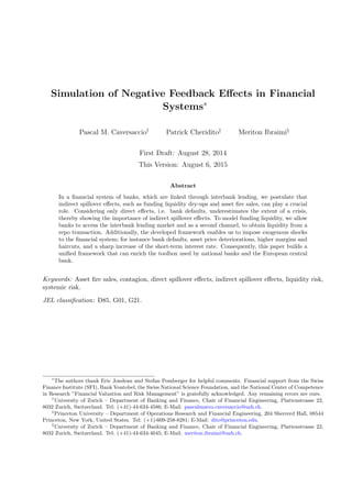
All scenarios have in common that at time t = 1 an asset price shock to the mortgage loans occurs.
The left column of Figure 2 is drawn by only allowing direct effects to occur, meaning that a bank
either directly gets insolvent due to the asset price shock or it gets insolvent as consequence of a
default of another bank. The right column of Figure 2 is drawn by additionally allowing for fire sales,
and in Figure 3 we further add indirect effects/shocks upon the first scenario. As Figure 2 shows,
when considering only direct effects the asset price shock added causes two banks to be insolvent
at time t = 2, and no further insolvencies occur afterwards. By adding only one indirect effect, i.e.
fire sales, we already obtain the insolvency of 7 banks in the time frame considered (see Figure 2).
Furthermore, from Figure 3 we can observe that imposing additional indirect spillover effects can
produce a full range of possible scenarios. Hence, the unified framework elaborated in this paper can
enrich the toolbox used by the responsible entity and can serve as an additional dimension for the
decision-making of a regulatory policy committee.
4 Conclusion
Our model provides a unified toolbox to generate stress scenarios for a system of banks which are
linked through overnight interbank lending. The strength of the model lies in the numerous shocks
that can be added to the system of banks, such as asset price shocks, defaults of banks, higher
haircuts/margins in repo borrowing and so forth. Furthermore, we also impose fire sales which are
amplifying crucial effects. Although our model is comprised of only a few, e.g. ten banks, the
extension to incorporate more banks is straightforward. Our numerical results show that indirect
effects play a major role in simulating the evolvement of a shock through a system of banks and
neglecting these indirect effects underestimates the extent of a crisis.
18

A Tables
Number and Size of Banks in Switzerland, by Type (2013)
Number of Banks Total Assets (CHF Bn) Proportion of Total Assets
Big Banks 2 1,322 46%
Cantonal Banks 24 496 17%
Foreign Banks 27 79 3%
Raiffeisen Banks† 1 174 6%
Regional and Saving Banks 64 106 4%
Private Banks 11 66 2%
Other Banks 154 607 21%
Total 283 2,849 100%
† The statistics cover all Raiffeisen banks, Raiffeisen Switzerland, and other group companies.
Table 1 – The Swiss banking structure in 2013. Source: Swiss National Bank.
19

Geographical and Structural Decomposition of the EU Banking Sector (2013)
Number of MFI Credit Institutions Number of Foreign Branches Total Assets of Domestic Banking Groups (EUR Bn) Total Assets of Foreign Subsidiaries and Branches (EUR Bn)
Belgium 39 64 469 491
Germany 1,734 109 6,457 278
Estonia 8 7 1 20
Ireland 431 34 275 514
Greece 21 20 356 13
Spain 204 85 3,271 217
France 579 91 6,154 189
Italy 611 81 2,405 227
Cyprus 74 27 41 26
Latvia 54 9 12 17
Luxembourg 121 37 90 628
Malta 27 3 13 38
Netherlands 204 39 2,252 181
Austria 701 30 788 301
Portugal 127 24 368 94
Slovenia 20 3 30 13
Slovakia 14 15 7 50
Finland 279 22 150 372
Euro Area 5,248 700 23,138 3,670
EU 7,726 978 - -
Table 2 – The geographical and structural composition of the EU banking sector in 2013. For comparability reasons, the euro area and EU aggregates
are based on a ﬁxed composition of 18 and 28 countries. Source: ECB Structural Financial Indicators, ECB Monetary Financial Institution (MFI)
Statistics, and ECB Financial Stability Committee (FSC) Consolidated Banking Data Statistics.
20

Random Variables at Time t = 1 States Distribution
Default of Bank n (Dn) {0, 1} Bin(1, pn)
Return of Collateral Assets RC
t rC
1 , rC
2 ∈ [−1, 1] Bin(1, q1)
Return of Reverse Repo Assets RRR
t rRR
1 , rRR
2 ∈ [−1, 1] Bin(1, q2)
Return of Residential Mortgages RM
t rM
1 , rM
2 ∈ [−1, 1] Bin(1, q3)
Return of Corporate Loans RCL
t rCL
1 , rCL
2 ∈ [−1, 1] Bin(1, q4)
Return of Derivatives RDV
t rDV
1 , rDV
2 ∈ [−1, 1] Bin(1, q5)
Return of Fixed Assets RF
t rF
1 , rF
2 ∈ [−1, 1] Bin(1, q6)
Repo Rate RR
n,t rR
n,1, rR
n,2 ∈ [0, 1] Bin(1, sn)
Aggregate Haircut (Ht) {h, h } ∈ [0, 1] Bin(1, v)
Individual Haircut (Hn,t) {hn, hn} ∈ [0, 1] Bin(1, vn)
Short-Term Interest Rate RS
t rS
1 , rS
2 ∈ [0, 1] Bin(1, w)
Table 3 – Description of the random variables in use for n ∈ [N] and t = 1.
Bank-Independent Parameter Values
r = 0.4
φtarget = 0.1
φ = 0.07
φR = 0.3
pC
0 = 17
pRR
0 = 18
pM
0 = 12
pCL
0 = 19
pDV
0 = 1
pF
0 = 3
H0 = 0.01
RR
n,0 = 0.01 ∀n ∈ [N]
RD
= 0.01
RA
= 0.02
τ = 1.054
λn,t = 0.3 ∀n ∈ [N] , ∀t ∈ [T]
Table 4 – The bank-independent parameter values employed in the simulation study.
21

w1 w2 w3 w4 w5 w6 w7 w8 w9
0.1 0.15 0.2 0.35 0.4 0.3 0.45 0.6 0.05
Table 5 – The risk weights employed in the simulation study.
Bank 1 Bank 2 Bank 3 Bank 4 Bank 5 Bank 6 Bank 7 Bank 8 Bank 9 Bank 10
Bank 1 0 960 95 664 792 430 59 562 271 640
Bank 2 599 0 184 261 315 72 513 856 398 680
Bank 3 186 362 0 899 824 138 926 757 888 832
Bank 4 720 188 295 0 287 677 821 85 246 825
Bank 5 240 34 981 191 0 895 632 252 1 381
Bank 6 595 692 33 882 960 0 335 804 655 52
Bank 7 500 375 15 748 870 572 0 901 769 626
Bank 8 52 457 907 350 512 637 691 0 268 162
Bank 9 85 305 405 507 599 534 248 990 0 424
Bank 10 609 445 764 546 366 496 601 469 244 0
Table 6 – The interbank loan matrix employed in the simulation study.
V C
n,0 V RR
n,0 V M
n,0 V CL
n,0 V DV
n,0 V F
n,0
Bank 1 409 459 628 255 512 202
Bank 2 328 323 733 751 362 750
Bank 3 578 313 579 712 635 459
Bank 4 399 206 793 414 722 642
Bank 5 320 709 304 255 306 260
Bank 6 718 368 577 399 437 250
Bank 7 631 441 611 240 441 670
Bank 8 398 630 300 252 514 754
Bank 9 768 711 289 634 305 337
Bank 10 554 467 285 446 449 471
V total 5,103 4,627 5,099 4,358 4,683 4,795
Table 7 – The initial volume of each asset for each bank employed in the simulation study.
22

ALIQ
n,0 AD
n,0 LS
n,0 LD
n,0 LL
n,0 Hn,0
Bank 1 9,479 4,417 10,996 6,148 7,550 0.01
Bank 2 2,654 3,231 10,083 7,730 8,278 0.02
Bank 3 5,184 3,588 12,666 7,496 6,295 0.01
Bank 4 4,464 5,345 11,413 7,470 7,398 0.03
Bank 5 14,115 4,430 10,466 7,571 8,229 0.001
Bank 6 15,599 5,356 13,953 7,641 8,696 0.02
Bank 7 12,896 4,208 11,053 7,266 7,302 0.06
Bank 8 12,133 5,389 10,303 7,495 6,908 0.02
Bank 9 13,951 3,622 14,068 9,862 6,376 0.02
Bank 10 10,610 5,932 11,989 7,693 7,499 0.002
Table 8 – The initial liquid– and deposit assets, short-term–, deposit–, and long-term liabilities, and bank-speciﬁc
haircuts employed in the simulation study.
D Hn,1 RR
n,1 RS
1 RC
1 RRR
1 RM
1 RCL
1 RDV
1 RF
1 H1
Bank 1 0 0.0166 0.02
Bank 2 1 0.0602 0.02
Bank 3 0 0.0263 0.02
Bank 4 0 0.0654 0.02
Bank 5 0 0.0689 0.08
Bank 6 0 0.0748 0.08
Bank 7 0 0.0451 0.02
Bank 8 0 0.0084 0.02
Bank 9 0 0.0229 0.02
Bank 10 0 0.0913 0.02
Aggregate 0.0002 -0.02 -0.04 -0.22 -0.01 -0.23 -0.015 0.01
Table 9 – The exogenous shocks to the interbank system with indirect spillover eﬀects.
23

B Figures
1990 1995 2000 2005 2010 2015
0
500
1000
1500
2000
2500
3000
3500
4000
4500
5000
5500
6000
Date
OutstandingRepoLiabilitiesin$Bn Total Repo Liabilities Reported in the Financial Accounts
Figure 1 – We plot the total repo liabilities in $bn reported in the financial accounts of the United States over
time. Source: Financial Accounts of the United States.
0 1 2 3 4 5 6 7 8 9 10
0
0.2
0.4
0.6
0.8
1
TTCR Time Evolution
t
TTCR
Bank 1
Bank 2
Bank 3
Bank 4
Bank 5
Bank 6
Bank 7
Bank 8
Bank 9
Bank 10
0 1 2 3 4 5 6 7 8 9 10
0
2
4
6
8
10
Number of Banks which are Liquid of Tier I
t
#Banks
0 1 2 3 4 5 6 7 8 9 10
0
0.2
0.4
0.6
0.8
1
TTCR Time Evolution
t
TTCR
Bank 1
Bank 2
Bank 3
Bank 4
Bank 5
Bank 6
Bank 7
Bank 8
Bank 9
Bank 10
0 1 2 3 4 5 6 7 8 9 10
0
2
4
6
8
10
t
#Banks
Figure 2 – On the top we depict the time evolution of the TTCR for the ten different banks. Additionally, on
the bottom the number of banks which satisfy the liquidity tier 1 are presented. Left column: This illustration
is produced by imposing a shock to the mortgage loans. The corresponding value can be found in Table 9.
Furthermore, we do not allow for asset fire sales, i.e. τ = 0. Right column: This illustration is produced by
imposing a shock of the mortgage loans and allowing fire sales, i.e. τ = 1.054. The corresponding value can again
be found in Table 9.
24

0 1 2 3 4 5 6 7 8 9 10
0
0.2
0.4
0.6
0.8
1
TTCR Time Evolution
t
TTCR
Bank 1
Bank 2
Bank 3
Bank 4
Bank 5
Bank 6
Bank 7
Bank 8
Bank 9
Bank 10
0 1 2 3 4 5 6 7 8 9 10
0
2
4
6
8
10
t
#Banks
0 1 2 3 4 5 6 7 8 9 10
0
0.2
0.4
0.6
0.8
1
TTCR Time Evolution
t
TTCR
Bank 1
Bank 2
Bank 3
Bank 4
Bank 5
Bank 6
Bank 7
Bank 8
Bank 9
Bank 10
0 1 2 3 4 5 6 7 8 9 10
0
2
4
6
8
10
t
#Banks
Figure 3 – On the top we depict the time evolution of the TTCR for the ten different banks. Additionally, on the
bottom the number of banks which satisfy the liquidity tier 1 are presented. Left column: This illustration is
produced by imposing a shock to the mortgage loans and a shock of the bank-specific repo rates, and additionally
allowing for fire sales, i.e. τ = 1.054. The corresponding values can be found in Table 9. Right column: This
illustration is produced by imposing several indirect spillover effects. The corresponding values can be again found
in Table 9.
25

References
T. Adrian and M. K. Brunnermeier. CoVaR. NBER Working Paper No. 17454, 2011.
G. Afonso, A. Kovner, and A. Schoar. Stressed, not frozen: The federal funds market in the financial
crisis. Journal of Finance, 66(4):1109–1139, 2011.
R. Albert, H. Jeong, and A.-L. Barabási. Error and attack tolerance of complex networks. Nature,
406(6794):378–382, 2000.
F. Allen and D. Gale. Financial contagion. Journal of Political Economy, 108(1):1–33, 2000.
P. Angelini, G. Maresca, and D. Russo. Systemic risk in the netting system. Journal of Banking &
Finance, 20(5):853–868, 1996.
M. L. Bech and K. Soramäki. Systemic risk in a netting system revisited. In Liquidity, risks and
speed in payment and settlement systems – a simulation approach. Bank of Finland Studies in
Economics and Finance, volume 31, pages 275–296. 2005.
M. K. Brunnermeier. Deciphering the liquidity and credit crunch 2007-08. Journal of Economic
Perspectives, 23(1):77–100, 2009.
M. K. Brunnermeier and P. Cheridito. Measuring and allocating systemic risk. Working Paper,
Princeton University, 2014.
O. Burrows, D. Learmonth, and J. McKeown. RAMSI: A top-down stress-testing model. Bank of
England Financial Stability Paper No. 17, 2012.
R. Cifuentes, G. Ferrucci, and H. S. Shin. Liquidity risk and contagion. Journal of the European
Economic Association, 3(2-3):556–566, 2005.
D. W. Diamond and P. H. Dybvig. Bank runs, deposit insurance, and liquidity. Journal of Political
Economy, 91(3):401–419, 1983.
D. Duffie. Systemic risk exposures: A 10-by-10-by-10 approach. In Risk Topography: Systemic Risk
and Macro Modeling. University of Chicago Press, United States, 2013.
26

L. Eisenberg and T. H. Noe. Systemic risk in financial systems. Management Science, 47(2):236–249,
2001.
M. Fleming and A. Sarkar. The failure resolution of Lehman Brothers. Economic Policy Review, 20
(2), 2014.
E. Gaffeo and L. Gobbi. Bilateral netting and contagion dynamics in financial networks. Working
Paper, University of Trento, 2015.
P. Gai and S. Kapadia. Contagion in financial networks. Proceedings of the Royal Society A: Math-
ematical, Physical and Engineering Science, 466(2120):2401–2423, 2010.
P. Gai, A. Haldane, and S. Kapadia. Complexity, concentration and contagion. Journal of Monetary
Economics, 58(5):453–470, 2011.
G. Gorton and A. Metrick. Securitized banking and the run on repo. Journal of Financial Economics,
104(3):425–451, 2012.
G. G. Kaufman. Bank contagion: A review of the theory and evidence. Journal of Financial Services
Research, 8(2):123–150, 1994.
Y. Leitner. Financial networks: Contagion, commitment, and private sector bailouts. Journal of
Finance, 60(6):2925–2953, 2005.
A. W. Lo. Complexity, concentration and contagion: A comment. Journal of Monetary Economics,
58(5):471–479, 2011.
K. Soramäki, M. L. Bech, J. Arnold, R. J. Glass, and W. E. Beyeler. The topology of interbank
payment flows. Physica A: Statistical Mechanics and its Applications, 379(1):317–333, 2007.
C. Upper. Using counterfactual simulations to assess the danger of contagion in interbank markets.
BIS Working Paper No. 234, 2007.
C. Upper and A. Worms. Estimating bilateral exposures in the German interbank market: Is there
a danger of contagion? European Economic Review, 48(4):827–849, 2004.
27

systemic_risk_final_version_ssrn

Recommandé

Recommandé

Contenu connexe

Tendances

Tendances (18)

En vedette

En vedette (11)

Similaire à systemic_risk_final_version_ssrn

Similaire à systemic_risk_final_version_ssrn (20)

systemic_risk_final_version_ssrn