properties, application and issues of support vector machine

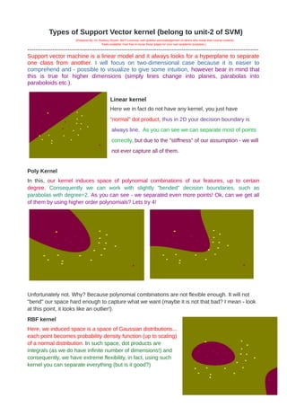
1. Types of Support Vector kernel (belong to unit-2 of SVM)
(Prepared By: Dr. Radhey Shyam, BIET Lucknow, with grateful acknowledgement of others who made their course contents
freely available. Feel free to reuse these pages for your own academic purposes.)
------------------------------------------------------------------------------------------------------------------------
Support vector machine is a linear model and it always looks for a hyperplane to separate
one class from another. I will focus on two-dimensional case because it is easier to
comprehend and - possible to visualize to give some intuition, however bear in mind that
this is true for higher dimensions (simply lines change into planes, parabolas into
paraboloids etc.).
Linear kernel
Here we in fact do not have any kernel, you just have
"normal" dot product, thus in 2D your decision boundary is
always line. As you can see we can separate most of points
correctly, but due to the "stiffness" of our assumption - we will
not ever capture all of them.
Poly Kernel
In this, our kernel induces space of polynomial combinations of our features, up to certain
degree. Consequently we can work with slightly "bended" decision boundaries, such as
parabolas with degree=2. As you can see - we separated even more points! Ok, can we get all
of them by using higher order polynomials? Lets try 4!
Unfortunately not. Why? Because polynomial combinations are not flexible enough. It will not
"bend" our space hard enough to capture what we want (maybe it is not that bad? I mean - look
at this point, it looks like an outlier!).
RBF kernel
Here, we induced space is a space of Gaussian distributions...
each point becomes probability density function (up to scaling)
of a normal distribution. In such space, dot products are
integrals (as we do have infinite number of dimensions!) and
consequently, we have extreme flexibility, in fact, using such
kernel you can separate everything (but is it good?)

2. Properties of SVM
1. Flexibility in choosing a similarity function
2. Sparseness of solution when dealing with large data sets - only support vectors are
used to specify the separating hyperplane
3. Ability to handle large feature spaces - complexity does not depend on the
dimensionality of the feature space
4. Overfitting can be controlled by soft margin approach
5. Nice math property: a simple convex optimization problem which is guaranteed to
converge to a single global solution
6. Feature Selection
SVM Applications
SVM has been used successfully in many real-world problems
- text (and hypertext) categorization
- image classification
- bioinformatics (Protein classification, Cancer classification)
- hand-written character recognition
Issues of SVM
This is a difficult question because SMVs are really versatile but I have found a couple of
curious cases where I think SVMs might be weak.
1. Data is not linearly separable and you have a lot of data.
When data is not linearly separable you have to use SVM with a kernel and having a lot
of data with the need of a kernel might lead to some performance issues. The option to
pre-compute a kernel matrix is infeasible and the computation of the kernel every time it
is needed might be expensive. There are approximations, the most famous one being
the Nystrom approximation but one has to be careful because a kernel SVM with the
Nystron approximation may not perform as well as some other classification algorithm.
2. You have only a few samples for some of your classes.
SVMs work better when you have plenty of samples for each class, if you only have a
few samples for some classes then KNN might work better than SVM. KNN can learn
very quickly a frontier while SVM takes a little longer but learns better more robust
frontiers because of the ability to maximize margin.
In brief:
SVMs do not perform well on highly skewed/imbalanced data sets.
SVMs are also not a good option specially if you have multiple classes.
SVMs are not efficient if the number of features are very huge in number compared to the
training samples.

3. Boundaries, hyperplanes, and slopes
In the lecture on support vector machines, we looked at different decision boundaries in 2D plots like
this:
In this image, line A has a larger margin than line B because it has more space separating it from the
nearest points. A also has a smaller ||w||, because when we learned about SVMs we learned that smaller
weights give larger margins.
You might be wondering how the weights w relate to the line that is shown. Earlier in the semester I said
that the weights represent the slope of the hyperplane, and you can visually see that B has a larger slope
in this plot -- so why doesn't B have larger weights?
Let’s discuss how the weights w relate to the slope of the decision boundary.
The lines you see on the plot above are not the hyperplane wTx. One realization to have is that a line
only has one independent variable (y=mx+b), whereas in this illustration, the instances actually have two
features, so x and y are both independent variables for the classifier. Instead of writing wTx, let's write
out the expanded equation for the hyperplane, using both x and y as the names of the
features: . (Remember that 'b' is the intercept, which I usually leave out of the
notation, but it's still there.)
This equation has two independent variables which makes it a plane, not a line. So why do you see just
a line in the plot of the decision boundary? The decision boundary isn't just the plane ,
but specifically the boundary . It's the "slice" of the plane where it passes through 0,
which forms a line. You can also see this algebraically by rewriting this as:

4. Now we have a line in the form of y=mx+b, where the slope corresponds to and the y-intercept
corresponds to . This line is the decision boundary that you see plotted. While the slope is based on
the weights , it's different from the slope of the full plane that defines the classifier
scores, .
This all applies to more dimensions. In general, there is a hyperplane of K dimensions that defines the
score of the classifier. The decision boundary is the set of points of that hyperplane that pass through 0
(or, the points where the score is 0), which is going to be a hyperplane with K-1 dimensions.
Now let me explain why smaller weights lead to larger margins.
Remember in an SVM, instead of one decision boundary wTx=0, we have two boundaries, wTx=1
and wTx=-1, illustrated like this:
Following the same steps from earlier in this post, let's rewrite the boundaries wTx=1 and wTx=-1 in full,
using x and y as the variables.

5. The positive boundary is:
The negative boundary is:
Both of these boundaries are lines with the same slope, so they are parallel. The margin is the distance
between these two parallel boundaries, which turns out to be:
(Why? See https://en.wikipedia.org/wiki/Distance_between_two_straight_lines)
Notice that is the Euclidean (L2) norm of the weights. With more than two features, this
distance generalizes to , which is what you learned in class. Therefore, a larger weight vector results
in a smaller distance between the two boundaries, aka a smaller margin.