control systems nptel lecture 53

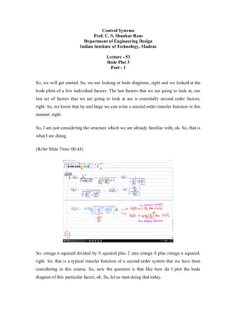
1. Control Systems
Prof. C. S. Shankar Ram
Department of Engineering Design
Indian Institute of Technology, Madras
Lecture - 53
Bode Plot 3
Part - 1
So, we will get started. So, we are looking at bode diagrams, right and we looked at the
bode plots of a few individual factors. The last factors that we are going to look at, our
last set of factors that we are going to look at are is essentially second order factors,
right. So, we know that by and large we can write a second order transfer function in this
manner, right.
So, I am just considering the structure which we are already familiar with, ok. So, that is
what I am doing.
(Refer Slide Time: 00:48)
So, omega n squared divided by S squared plus 2 zeta omega S plus omega n squared,
right. So, that is a typical transfer function of a second order system that we have been
considering in this course. So, now the question is that like how do I plot the bode
diagram of this particular factor, ok. So, let us start doing that today.

2. So, this can be rewritten as 1 divided by I just divided by omega n square in both
numerator and denominator. So, essentially I will get it as S by omega n whole square
plus 2 zeta by omega n S plus 1, right. So, that is what will happen, correct. So, if I
divide both numerator and denominator by omega n squared, so immediately what is
going to happen is that like if I calculate G of j omega, so what would I get? I would get
1 divided by 1 minus omega by omega n whole square plus 2 zeta omega by omega n j,
right. So, that is what I will have, ok.
So, 2 zeta omega by omega n, right. So, that is what we will have as the sinusoidal
transfer function. So, once I have this, what can I how can I write the magnitude of this
particular factor? So, I can say this is going to be 1 divided by square root of the real
path square. So, the real path square is going to be 1 minus omega by omega n whole
square and this I have 2 square. That is a real part. Then, I take the square of the real part
plus the imaginary part squared so 2 zeta omega by omega n whole square, right.
So, that is what I do, ok. So, then what will be the phase of the sinusoidal transfer
function? That is going to be minus tan inverse of 2 zeta omega by omega n divided by 1
minus omega by omega n whole square, right. So, that is what we get as the phase, right
of this particular factor, right. It is pretty straightforward algebra, ok.
So, now let us look at the magnitude will once again we will follow the same process as
we did in the previous class with the first order factor. So, let us look at the magnitude of
this factor and then, let us try to figure out what are the asymptotes for this particular
factor, right. So, we can immediately see that the magnitude of this particular factor in
decibels is going to be minus 20 log to the base 10 square root of 1 minus omega by
omega n whole square square plus 2 zeta omega by omega n square, ok.
So, that is what will happen, ok. So, this is going to be in decibels, right. So, what will
happen as omega is very small. What do you think will happen to this magnitude when
omega is very small when compared to omega n let us say. So, the magnitude of G of j
omega you can immediately see that will tend to 0 decibels as omega is much smaller
than omega n. Why am I taking omega n? It is because we have omega divided by omega
n, right as a term, right.

3. So, I have to compare the frequency in relation to omega n, right. So, when the
frequency of interest becomes much less than omega n which is the natural frequency of
the system, we can see that omega by omega n becomes very small. So, obviously,
omega by omega n whole squared also will be pretty small, right. So, in the square root
term, I will effectively end up with 1. So, I am essentially going to take log of 1, so that I
will get zero decibels, right. So, that is what is going to happen when I have omega much
lower than omega n and what is going to happen when omega is much greater than
omega n, ok. So, let me erase this and say when omega is much less than, ok. What do
you think happens when omega is much greater than omega n?
Obviously, omega by omega n is now going to be much greater than 1, ok. So, now
within this first term if you look at it, you have 1 minus omega by omega n square. So,
that will effectively become minus omega by omega n squared, but you are squaring it.
So, the first term is going to be like omega by omega n to the power 4, right.
The second term is 2 zeta omega by omega n whole square. Now, which term is going to
dominate? First term, right that is omega n by omega by omega n to the power 4. So,
now when you take the square root of omega by omega n to the power 4, what do we
get? We get omega by omega n whole square, right. So, then if I take the logarithm of
that, what will I get?
Student: 40 log.
I am going to get minus 40 log to the base 10 omega divided by omega n. Is it clear?
How? Of course, this is in decibels, right. So, is it clear how we got minus 40 log omega
by omega n because I am sorry what is it?
So, you can see that the first term tends to omega by omega n to the power 4, the second
term is like omega by omega n whole square. Just think that omega by omega n is 10
power 3. So, the first term is going to be like 10 power 12, right. The second term is
going to be like 10 power 6. So, the first term is obviously dominate, right. You take the
square root, you are going to get omega by omega n squared.
So, log of omega by omega n squared is 2 log omega by omega n. So, there is already a
minus 20, you multiply it by 2, you get minus 40, right. So, that is why the magnitude

4. tends to minus 40 log to the base 10 omega by omega n decibels when omega is much
greater than omega n. So, obviously we already know that this one is going to be the low
frequency asymptote, right and this one is going to be the high frequency asymptote just
like what we did yesterday, right.
So, this is going to be the high frequency asymptote, ok.
(Refer Slide Time: 08:26)
So, that is what we will have here. Now, once again a set of questions there like the first
one is, where do the two asymptotes intersect? Where do you think the two asymptotes
intersect each other? Omega equals omega n. We can immediately figure out the answer
as omega equals omega n. Why? It is because you see that when you substitute omega
equals omega n in the high frequency asymptote, you get zero decibels, right.
So, essentially zero decibel line is the low frequency asymptote. So, essentially the two
asymptotes intersect at omega equals omega n, right. So, consequently omega equals
omega n is the corner frequency, right for this particular factor, right the second order
term, ok. The natural frequency is the corner frequency, ok. Is it clear because that is the
frequency at which the two asymptotes intersect?
So, the second question that we need to ask ourselves is that what is the slope of the high
frequency asymptote? What do you think is a slope? So, the high frequency asymptote is
minus 40 log to the base 10 omega by omega n, right. So, how do we figure out the

5. slope? Let us say you go one decade further right from omega. So, instead of omega, you
substitute ten times omega. What do we get? So, immediately we see that minus 40 log
to the base 10, 10 times omega by omega n that is going to be equal to what? Of course,
in decibels that is going to be equal to minus 40 decibels, all right minus 40 log of log to
the base 10 of omega by omega n in decibels, right. So, what is the slope?
So, slope of the high frequency asymptote is going to be minus 40 decibels per decade,
right. So, is equal to minus 40 decibels per decade, ok. That is what matters. So, please
note that here the slope is going to be slope of the high frequency asymptote is minus 40
decibels per decade. So, as frequency increases, the magnitude decreases like minus 40
decibels per decade, ok. That is important, ok.
Now, another question which we are going to ask ourselves is that when is the magnitude
of G of j omega a maximum or at what frequency ok? So, in other words, you know like
at what frequency is the magnitude of G of j omega a maximum, right? So, that is a
question we are going to ask ourselves. So, let us try to answer that.
(Refer Slide Time: 11:57)
So, what is the magnitude of G of j omega. It is going to be 1 divided by square root of 1
minus omega squared by omega n square whole square plus 2 zeta omega by omega n
whole squared, right. So, this is the magnitude, right.

6. So, now when is this going to be a maximum? Of course, how can I find out at what
frequency this is going to be a maximum i differentiate equated to zero and then, like
take the second derivative figure out where it is, the second derivative is negative for a
maximum right, but here I can use a simpler method because this in the numerator is 1,
right. So, I will have a maximum where the denominator is going to be a minimum. I can
even what you say remove the square root, right.
So, at whatever frequency the term within the square root in the denominator is a
minimum, that is the frequency at which the magnitude of G of j omega is going to be
maximum, right. So, let us say we call f of omega some f of omega as 1 minus omega
squared by omega n square whole square plus 2 zeta omega by omega n whole square.
Now, if we take the derivative, the first derivative of f of omega with respect to omega,
what do we get? We get two times 1 minus omega squared by omega n squared times 2
omega divided by omega n square, right. So, first I just then I have a minus sign, right.
So, when I take the derivative of the term within the square, right I will get a minus sign,
right. So, let me put this minus sign here, and then, what will I have here? I will have
essentially 2 times 2 zeta by omega n, correct. Then, what will I have? I will have 2 zeta
by omega n, correct. So, this should be equal to 0, ok.
So, now if I process this, what will I get for omega? Can you calculate and tell me? So,
you can see that I immediately have this omega n squared cancelling off with this omega
n. Let us say this 2, this 2 cancelling off these 2, right. So, what will I have? I will have
minus 1 by omega squared divided by omega n squared. Obviously, omega is non-zero,
right. So, of course I can have two solutions, ok. We will come to that shortly you know
like. So, plus 2 zeta times omega is equal to 0, right.
So, this has two solutions, right. I just simplified this and wrote it. So, obviously you
know like omega is 0 is one particular solution, right. It can be 0, right or the term within
the square bracket is 0. That will imply that 2 zeta is going to be equal to 1 minus omega
squared by omega n square, ok. Sorry this should be 2 zeta squared, right correct. I think
I missed a zeta here, right. So, 2 zeta square. So, this will tell me that omega can also be
omega n times square root of 1 minus 2 zeta squared, ok. Correct? I am just rearranging
the terms and doing some simple algebra.

7. Now, when will this solution be a real number because we are dealing with frequencies,
right. See I want a positive real number, right. When will this solution exist? This exists
only when 1 minus 2 zeta squared is greater than 0 or in other words, zeta should be less
than 1 over root 2, right 0.70 so on, right. 1 over root 2 is 0.70 approximately, right.
Student: (Refer time: 17:46).
Sorry.
Student: (Refer time: 17:47).
But, anyway zeta is a positive number, ok. Of course, when we started off, I have to say
that zeta and omega n are a positive parameter. You are right in general, but since we are
essentially dealing with systems where zeta and omega are not positive, this is what I
have, right.
(Refer Slide Time: 17:13)
.
So, this frequency omega r is called as the. Have you encountered this frequency before?
This is what is called as a resonant frequency, and of course, it exists only when zeta is
greater than 0 and less than 1 over root 2, otherwise it does, for zeta greater than 1 over
root 2 omega tending to 0 will give you the maximum value that is the 0 decibel value,
but for zeta between 0 and 1 over root 2, you know like you have the resonant frequency

8. basically giving you the maximum value of the amplitude or magnitude of the sinusoidal
transfer function for the second order factor, ok.
So, what is this resonant frequency? See we had we already defined a couple of
frequencies, right. So, what was natural frequency? See you take a second order system
let us say you remove the damping, right then you give a perturbation, the frequency at
which the undamped system oscillates is what is called as the natural frequency, right
and also, if you look at it, let me write it as an aside if you look at an undamped second
order system.
So, undamped second order system, the plant transfer function is going to be like omega
n squared divided by s squared plus omega n squared. Do you agree? So, that is how we
got, we have the visualization right of natural frequency, you give a perturbation, or
essentially then the frequency at which the output will oscillate is essentially the natural
frequency, but if you also give an input which is essentially let us say sin or cosine of
omega n, let us say you give sin omega n t. What is going to happen to the output? We
are going to get omega n square times omega n divided by s squared plus omega n square
whole square, right. So, once I have this, what will happen? I think we already discussed
these things, right. What would happen once I have s squared plus omega n squared
whole square? I am going to have t sin t or t cos t, right term.
So, consequently what will happen to the magnitude of Y of t? It will go to infinity, right
as t tends to infinity, right. So, this is another visualization of a natural frequency that is
if you have an undamped second order system and you give an input which essentially
which has a frequency equal to the natural frequency, the output will just explode to
infinity, ok. That is natural frequency, ok. That was the first data what was undamped
natural frequency. Sorry? Sorry, this is the, sorry this is the natural frequency. What is
damped natural frequency?
Damped natural frequency was the frequency at which the damped second order system
oscillator, right when the damping ratio was between 0 and 1 in response to an step input,
right. So, we looked at omega d if you remember, right. So, there are three natural
frequencies of interest. So, the first one is natural frequency which by definition
corresponds to the undamped system, right.

9. The second one was the damped natural frequency which essentially corresponds to an
under damped second order system, and the damped natural frequency is omega n times
square root of 1 minus zeta square, right. So, physically what is say notion of this
damped natural frequency? We have a stable second order system. You give a step input,
the frequency at which the corresponding output would oscillate is what is called as the
damp natural frequency and even if you give a sinusoidal input equal to the damped
natural frequency, the system output would be bounded because you have an under
damped stable second order system, ok. No doubt about it.
Now, the third frequency is the resonant frequency omega r. So, what is this omega r,
which is essentially omega n times square root of 1 minus 2 zeta square. This essentially
means that I have a stable under damped second order system with damping ratio
between 0 and 1 over root 2. If I have such a system, this is the frequency at which the
amplitude of the corresponding sinusoidal transfer function will be maximum, ok. So,
that is the implication, ok.
So, in other words, if you give a sinusoidal input equal to whose frequency is equal to
omega r, you would get the maximum amplification of the input because p the amplitude
of the transfer function is maximum with this frequency. That is what we have seen right.
Isn't it? So, that is the physical meaning of the resonant frequency. Resonant frequency
resonance and resonant frequency still correspond to a stable second order system, but
then it is bad in practice because of the amplification of the oscillations because what is
this physically? What is this magnitude of G of j omega?
If you recall our derivation, the output steady state output was u magnitude of the input
times magnitude of G of j omega. So, the output is also going to be a sinusoid, but the
input amplitude is going to be multiplied by the magnitude of the sinusoidal transfer
function. So, imagine frequency at which the magnitude of the sinusoidal transfer
functions of the maximum.
So, the output amplitude which is a sin wave that will also be a maximum there; it is still
bounded mathematically ok, but physically it may create issues, ok. The system is still
stable no doubt about it right, but then resonance can lead to oscillations of reasonably
high magnitude which can cause structural damage, ok. So, one famous example you

10. know like which is typically given to illustrate this is what is called as Tacoma Narrows
Bridge Collapse, right.
So, you please search online and watch the video Tacoma Aqus Narrows Bridge, ok. So,
you will see that the wind essentially excited the resonant frequency and the entire bridge
swayed, ok. Yes, mathematically it is bounded, the amplitude is bounded, but what
happened the structure field, because of the excessive oscillations, right. So, that is what
happened. So, just watch the video, right.
So, that is the resonant frequency, right. So, that is why I just wanted to do this analysis
to convey the difference between natural frequency, damped natural frequency and
resonant frequency. I hope the physical meaning is clear for each frequency because this
understanding is extremely critical and we want to analyze second order systems, right.
So, please know that resonant frequency once again is applicable only for those second
order systems where the damping ratio is between 0 and 1 over root 2, ok. I hope this
point is clear, right but we are not done with the derivation yet. As homework, what I
want you to do is that you have to take the second derivative and then, ensure that f of
omega f double prime omega is going to be positive at this frequency, right. That I leave
it for your homework because whenever you do maximization or minimization, you need
to do both steps. I cannot leave it hanging like this, but I am going to leave it to your
homework, ok.
So, as homework evaluate the second derivative, and comment ok. So, that is essentially
your homework. Obviously, you will see that at this resonant frequency, the second
derivative is positive. So, as a result the magnitude of G of j omega will be a maximum,
because magnitude of G of j omega is 1 by f omega, right. So, that is why when f omega
is minimum, magnitude of G of j omega will be a maximum, ok. So, that is what we will
have, ok.
So, please do that and we can easily show that, this is also I am going to leave it as
homework.

11. (Refer Slide Time: 27:08)
So, the magnitude of G of j omega, the maximum value which is the magnitude of G of j
omega at omega equals omega r is going to be 1 divided by 2 zeta times 1 minus zeta
square, ok. So, this you just need to plug in the value of omega in that expression, ok.
You will easily get it and the phase of G of j omega at omega equals omega r, you will if
you substitute in that equation for the phase, you will get it as minus tan inverse square
root of 1 minus 2 zeta squared divided by zeta. Immediately you see that the maximum
magnitude and the phase at the corresponding resonant frequency depend on the
damping ratio, the zeta, ok.
So, that is what we have, ok. You can just substitute and then, very straightforward you
just substitute and then figure out.