1. Control Systems
Prof. C. S. Shankar Ram
Department of Engineering Design
Indian Institute of Technology, Madras
Lecture - 55
Bode Plot 4
Part - 1
So, we had been we have been looking at bode diagrams right. So, and yesterday we
saw; what was the difference between a minimum phase and a non-minimum phase
system right as far as the asymptotes asymptotic value of the magnitude plot and the
phase plot were concerned. So, today let me generalize it you know like let us say in
general you have a transfer function G of s which is a ratio of n of s and d of s. And let
us say the numerator polynomial is of order m the denominator polynomial is of order n.
So, what is going to happen is that; like if you have a minimum phase system that means
that of course I am what to say assuming that you know all the zeros are in the left of
complex plane by a minimum phase system. You will see that we can generalize the
asymptotic value of the phase plot. So, let me write down some general statements you
know like and then like we will discuss them.
(Refer Slide Time: 01:25)
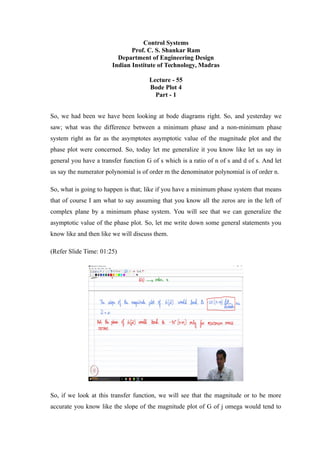
So, if we look at this transfer function, we will see that the magnitude or to be more
accurate you know like the slope of the magnitude plot of G of j omega would tend to
2. minus 20 times n minus m decibels per decade as omega tends to infinity ok. This so this
is going to be true for both minimum phase and non-minimum phase systems ok. So,
essentially n minus m is the relative degree of the transfer function, right. So, the slope of
the magnitude plot is always going to tend to a value of minus 20 times n minus m
decibels per decade ok. So, irrespective of whether we have a minimum phase system or
a non-minimum phase system.
(Refer Slide Time: 02:31)
So, this is something we can check from the previous example right. So, what did we do
in the last class? So, we immediately saw that what to say the magnitude plots
magnitudes were essentially the same. And if you look at it, you know like this is like 1
plus t s and 1 plus t 1 s right. So, if you consider this right, so you have two factors right
this I can rewrite as 1 plus t s times of 1 plus 1 divided by 1 plus t 1 s, right.
So, we already know from the building blocks that as omega tends to infinity what is the
slope of 1 plus t s, it is going to be 20 decibels per decade right. And what is the slope of
high frequency asymptotes slope, you know like it is going to be minus 20 decibels per
decade for 1 divided by 1 plus t 1 s right. So, as omega tends to infinity right, so as you
go to higher frequency so what is going to be the next slope this is a going to be a sum so
which is essentially 0.
So, you can see that in this case n was 1, m was also 1 right. So, you can immediately see
that the n minus m is 0 that is why in the previous example you know like would have a
3. slope of zero decibels per decade at high frequency essentially the magnitude curve will
flatten out right. So, that is what will happen this is true for a minimum phase and non
minimum phase systems. But, the phase of G of j omega would tend to minus 90 degrees
times n minus m only for minimum phase systems. So, this is an important
distinguishing feature ok. So, only for minimum phase systems you know like would we
have the slow the phase of the sinusoidal transfer function tending to minus 90 degrees
times n minus m ok. Once again we could observe it from the previous example right.
So, in the previous example, once again n was 1, m was 1. So, what happened we saw
that the phase tends went to zero degrees right as omega tends to infinity for the
minimum phase system, because n minus m is 0 for the previous example. So, you one
can immediately observe the generalization. But then like for a non-minimum phase
system, we saw that it went to value different from minus 90 degrees times n minus 1 ok,
so that is what happens.
So, this is something which we will use later, you know like there is if you conduct
experiments. And then like if you happen to plot get the magnitude plot and the phase
plot right, one could use this information to figure out the relative degree of the transfer
function. Because for the magnitude plot, you look at the slope of the high frequency
curve you will get n minus m right. So, you will know; what is the relative degree of the
transfer function correct. So, because the slope is going to be minus 20 times n minus m
are decibels per decade right.
And then like you look at the high frequency a value for the phase, you will get you will
be able to determine whether it is a minimum phase system or a non-minimum phase
system right. So, that information is something you can obtain right. So, we will see you
know like when we do a case study slash project you know like towards the end, we will
look at this thing. So, that is something we will do later on, fine.
4. (Refer Slide Time: 06:43)
So, let us essentially now do one example today. So, that like where we construct the
bode plot of a transfer function from start. So, this will illustrate the entire process like as
to how to construct the magnitude plot and the phase plot. So, let us do an example today
right. So, let us consider a transfer function which is of the form let us say s divided by s
plus 1 times s plus 10 ok. So, let us say I consider this transfer function right. So, I want
to plot the bode diagram for this particular transfer function.
So, obviously, we need to rewrite this transfer function in terms of the factors that we
have learned till now right. So, how can I rewrite it in terms of in the structure of factors
that we have learned till now, is it already in that structure, not really right. So, what
should I change, see the s plus 10 term in the denominator, I should make the constant
term as 1 right.
So, what do I do I just pull 10 out right? So, if I do that what is going to happen I am
going to get this right s by 10 plus 1? So, this will give me 0.1 s divided by s plus 1 times
0.1 s plus 1. Do you agree right? So, this essentially means that I have four factors a
constant 0.1 a s term and then a 1 by s plus 1 term and then a 1 by 0.1 s plus 1 right. So, I
have I have to plot the individual bode plots of these four factors and then get the net
bode diagram right, so that is what I need to do.
So, look if I start looking at each term, if I take a look at 0.1 what can I say about its
magnitude in decibels, so if I take logarithm and multiply it by 20, how many decibels
5. will I get? What is log of 0.1 to the base 10? Minus 1, right; so essentially I am going to
get the magnitude as minus 20 decibels right, so that is going to be constant. What about
its phase? Zero right, anyway it is on the positive real axis ok, so that is what I will have.
So, then the second factor is s what is its magnitude in decibels? If you recall, it is a 20
log omega right. So, you have a straight line with the slope of 20 decibels per decade
right. So, what is the phase, what is its phase, what is the phase of the s term plus 90
degrees right? So, we discuss this.
So, the third term is 1 by s plus 1, this is of term of the form 1 by t s plus 1. So, so
essentially we can draw the low frequency asymptote and the high frequency asymptote.
What is the corner frequency of this term here T is capital T is 1. So, 1 by capital T is a
corner frequency right. So, what is a corner frequency 1 right; so one radians per second
is a corner frequency for this particular term.
So, then the fourth term is going to be 1 divided by 0.1 s plus 1 right. So, what is its
corner frequency? Here you see that t is 0.1. So, one by t is going to be ten. So, 10
radians per second is the corner frequency right. I hope it is clear how we got these
values right for the corner frequency. So, these are the four blocks we just need to plot
the magnitude plot and the phase plot for these four terms and then add them that is it
that is all we need to do right.
(Refer Slide Time: 11:21)
6. So, let us let us start from the magnitude plot. So, let me start with the magnitude plot.
So, let us say I draw so omega. So, let us say I consider of course, 1 and 10 are going to
be my corner frequency. So, I consider a frequency range typically you know one decade
above and one decade below the corner frequencies you know like that is that is typically
the choice of a range of frequencies at b by and large consider it is a rule of thumb you
can go for a larger range also no issues with that.
So, on the abscissa we are sorry on the ordinate we are going to plot the magnitude. So,
vertical axis we will have the thing in decibels. So, let us say you know like I have 0
decibels, or minus 20, minus 40, minus 60 plus 20 and so on ok. So, these are my values.
So, let us plot each term one by one ok. So, let us start with s. So, I am just going to use a
same colour code you know like as what I wrote for the four factors, so that it is obvious
what I am plotting right. So, let us first take the constant term right 0.1. So, what is the
magnitude plot of the constant term? You see that the magnitude of 0.1 is minus 20
decibels right so obviously that that will remain the case irrespective of the frequency.
So, what can you say about the magnitude plot of 0.1, it is just going to be a just a
horizontal line at minus 20. So, this is the magnitude plot of 0.1 at minus 20.
Now, what happens to the next factor, the next factor is s so that essentially has
magnitude plot of a straight line with a slope of plus 20 decibels per decade if you recall
what we had right. So, for s the magnitude is 20 log to the base 1- omega. So, at omega
equals 1, what is the value of this particular magnitude, it is going to be 0.
So, let us say I plot at omega equals 1, so that is going to be 0; at omega equals 10, I am
going to have the value as 20. So, and at omega equals 0.1, I am going to have the value
as minus 20. So, I am just plotting the values. So, the magnitude plot of the s factor is
going to be a straight line ok. So, essentially I am sorry I am just erasing this a straight
line which passes through these points and which has a slope of plus 20 decibels per
decade ok. So, this is the magnitude plot of s. So, this has a slope of 20 decibels per
decade so that is the second magnitude plot, alright.
Now, we go to the third factor 1 by s plus 1. So, if you recall what we had about the
factors or the form 1 by t s plus 1 right so once again as we told as we discussed you
know like when we are drawing things by hand in excess example problems in
homeworks and exams, I want it you to only draw the asymptotes ok. You do not need to
7. apply the correction as a first cut plot. Of course, in real life you need to apply the
correction and get the actual plots. But nowadays you know like if you use the command
bode in MATLAB you will get what to say the bode plot itself right. So, you just check
out the command bode in MATLAB.
So, let us plot bode diagram for the asymptotes for 1 by s plus 1. So, what is a low
frequency asymptote in the magnitude plot for 1 by s plus 1, 0 decibels. So, if you recall
what we discussed, so we are going to have till the corner frequency of one. So, one is
my corner frequency. So, I am going to have zero decibels as my low frequency
asymptote. And what is going to be my high frequency asymptote that is going to be a
straight line with a slope of minus 20 decibels per decade.
So, how do I plot it let us say I take a frequency of 10, I mark as minus 20 then I can plot
the high frequency asymptote with the slope of minus 20 decibels per decade. So, this is
bode diagram for 1 divided by s plus 1. So, of course, when you draw you need to
essentially mark all the factors and also the slopes and other critical points like what I am
doing here ok. So, I am also indicating the slope right as minus 20 decibels per decade.
So, this is the third factor 1 by s plus 1.
Now, we need to look at the fourth factor which is 1 divided by 0.1 times s plus 1 right.
So, we know that the corner frequency is going to be 10. So, once again the low
frequency asymptote is going to be the zero decibel line so and then like that is going to
extend till so the corner frequency of 10.
So, let us say the corner frequency is somewhere here ok, till 10 we are going to have the
zero decibel line as the low frequency asymptote. Once again what is going to be the
high frequency asymptote, a straight line with a slope of minus 20 decibels per decade.
How can I do that? At 10 radians per second the value is 0 decibels; if I want a slope of
minus 20 decibels per decade what is a frequency 1 decade above 10, 100 right. At that
frequency I should have a value of minus 20.
So, at 100, I find out I mark minus 20 as my magnitude. And then like what I do is that I
just draw a line that passes through this point ok, so that is my magnitude plot of course
asymptotes further factor 0.1 divided by 0.1 s plus 1. Even this has a slope of minus 20
decibels per decade ok, so that is this slope.
8. Now, we have plotted all the four graphs right. Now, what we need to do we just need to
add them. So, what will be the net sum of all these four terms, what do you think will
happen? How can I add them? So, you see that the s term is going to affect throughout all
frequencies right. And the minus 20 decibels per decade term also will affect throughout
all frequencies. And the 1 by s plus 1 term and 1 by 0.1 s plus terms the effects will come
at the corresponding starting from the corresponding corner frequencies, because till
these corner frequencies the contribution is zero decibels right.
So, what will happen, I have this plot for this s term which essentially is a straight line of
the slope of plus 20 decibels per decade, but that is going to be shifted down by minus 20
decibels. Why, because I have the factor of 0.1 right. So, let me start by plotting the bode
plot till the corner frequency of 1. So, what is going to happen I need to shift the graph of
the s term by minus 20 decibels ok, so that is what I need to do. So, if I shift by minus 20
at the frequency of 0.1, the value will become minus 40. And the value of 1, it is going to
become minus 20 so that is what is going to happen to 0.1 times s right till the corner
frequency of one.
So, what I do is that, I am going to use the red solid line to essentially draw the bode
diagram of the total transfer function the net transfer function. So, this is what is going to
happen to my; what did I do. So, this is what is going to happen to the bode diagram of
the transfer function at low frequencies till the corner frequency of plus 1.
Now, what happens at plus 1? At plus 1 the one by s plus 1 terms starts contributing a
high frequency asymptote with a slope of minus 20 decibels per decade is not it. Now,
you have so let me let me essentially write in maybe pink what I am doing ok, till 1 till
what to say omega less than 1, what I am plotting is 0.1 s, 0.1 times s right because that
is what will contribute to the magnitude plot. Between omega 1 and 10, we will have 0.1
times s times s plus 1 right.
Now, s will have a slope contribute a slope of plus 20 decibels per decade 1 divided by s
plus 1 will contribute a slope of minus 20 decibels per decade, both will the slopes will
just cancel off. So, what will I be left with, I will just very left to the horizontal line of
the same value. So, in essence my magnitude will remain constant oops right. So, my
magnitude will remain constant at minus 20 decibels per decade till I reach the slope of a
9. sorry till I reach the corner frequency of minus sorry till I reach a corner frequency of 10
right. I hope it is clear how we got this.
Now, what will happen after 10? From omega greater than 10, I will have all the terms
coming into play right. So, I will have this 0.1 s plus 1 also starting to contribute right.
And what will be the contribution of 0.1 s plus 1; it will contribute a slope of minus 20
right. So, in essence what is going to happen is that at 100, I should have minus 40. So, I
think let me just quickly erase this so that I draw it properly.
So, just bear with me for a second. See, please use a scale to draw the bode plot cleanly
ok. So, I am just drawing freehand. So, as a result you know like there is some offset. So,
this is the bode diagram for the factor 1 divided by s plus 1 right. So, so the slope was
minus 20 decibels per decade this was the factor 1 divided by s plus 1.
So, what is going to happen, now for the entire transfer function it is going to have a
slope of minus 20 decibels per decade. So, it is going to go along the same line so that is
what happens here right. So, the red curve the red solid line is for this entire transfer
function, the magnitude plot of the entire transfer function ok, is it clear.
What I did? See I just read through that green line and so that it is to scale ok, see
obviously, the high frequency asymptote of one by s plus 1 and 1 divided by 0.1 s plus 1
should be parallel right because their slopes are the same right so that is why just redrew
it to scale so that is what I have done here that is it.
So, I hope it is clear how we got this what to say the net curve right for the magnitude
plot. So, here in the low frequency region, the slope is going to be plus 20 decibels per
decade for the thing. And in the high frequency region, the slope is going to be minus 20
decibels per decade. So, this is how we get the magnitude plot of the complete transfer
function ok. Is it clear, fine?