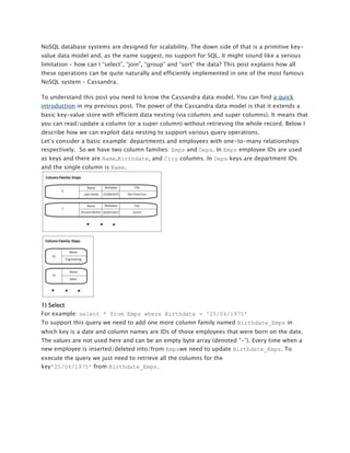
1. NoSQL database systems are designed for scalability. The down side of that is a primitive key-
value data model and, as the name suggest, no support for SQL. It might sound like a serious
limitation – how can I “select”, “join”, “group” and “sort” the data? This post explains how all
these operations can be quite naturally and efficiently implemented in one of the most famous
NoSQL system – Cassandra.
To understand this post you need to know the Cassandra data model. You can find a quick
introduction in my previous post. The power of the Cassandra data model is that it extends a
basic key-value store with efficient data nesting (via columns and super columns). It means that
you can read/update a column (or a super column) without retrieving the whole record. Below I
describe how we can exploit data nesting to support various query operations.
Let’s consider a basic example: departments and employees with one-to-many relationships
respectively. So we have two column families: Emps and Deps. In Emps employee IDs are used
as keys and there are Name,Birthdate, and City columns. In Deps keys are department IDs
and the single column is Name.
1) Select
For example: select * from Emps where Birthdate = '25/04/1975'
To support this query we need to add one more column family named Birthdate_Emps in
which key is a date and column names are IDs of those employees that were born on the date.
The values are not used here and can be an empty byte array (denoted “-”). Every time when a
new employee is inserted/deleted into/from Empswe need to update Birthdate_Emps. To
execute the query we just need to retrieve all the columns for the
key'25/04/1975' from Birthdate_Emps.

2. Notice that Birthdate_Emps is essentially an index that allows us to execute the query very
efficiently. And this index is scalable as it is distributed across Cassandra nodes. You can go
even further to speed up the query by redundantly storing information about employees (i.e.
employee’s columns from Emps) in Birthdate_Emps. In this case employee IDs becomes names
of super columns that contain corresponding employee columns.
2) Join
For example: select * from Emps e, Deps d where e.dep_id = d.dep_id
What does join essentially mean? It constructs records that represent relationship between
entities. Such relationships can be easily (and even more naturally) represented via nesting. To
do that add column familyDep_Emps in which key is a department ID and column names are IDs
of the corresponding employees.
3) Group By
For example: select count(*) from Emps group by City
From implementation viewpoint Group By is very similar to select/indexing described above.
You just need to add a column family City_Emps with cities as keys and employee IDs as
column names. In this case you will count the number of employees on retrieval. Or you can
have a single column named count which value is the pre-calculated number of employees in
the city.

3. 4) Order By
To keep data sorted in Cassandra you can use two mechanisms: (a) records can be sorted by
keys using OrderPreservingPartitioner with range queries (more on this in Cassandra:
RandomPartitioner vs OrderPreservingPartitioner). To keep nested data sorted you can use
automatically supported ordering for column names.
To support all these operations we store redundant data optimized for each particular query. It
has two implications:
1) You must know queries in advance (i.e. no support for ad-hoc queries). However, typically in
Web applications and enterprise OLTP applications queries are well known in advance, few in
number, and do not change often. Read Mike Stonebraker convincingly talking about that. BTW,
Constraint Tree Schema, described in the latter paper, also exploits nesting to organize data for
predefined queries.
2) We shift the burden from querying to updating because what we essentially do is supporting
materialized views (i.e. pre-computed results of queries). But it makes a lot of sense in case of
using Cassandra as Cassandra is very much optimized for updates (thanks to eventual
consistency and “log-structured” storage borrowed from Google BigTable). So we can use fast
updates to speed up query execution. Moreover, use-cases typical for social applications are
proven to be only scalable with push-on-change model (i.e. preliminary data propagation via
updates with simple queries – the approach taken in this post) in comparison with pull-on-
demand model (i.e. data are stored normalized and combined by queries on demand – classical
relational approach). On push-on-change versus pull-on-demand read WHY ARE FACEBOOK,
DIGG, AND TWITTER SO HARD TO SCALE?
Consideration for NoSql
Do you need a more flexible data model to manage data that goes beyond a rigid
RDBMS table/row data structure and instead includes a combination of structured,
semi-structured, and unstructured data?
• Do you need continuous availability with redundancy in both data and function
across one or more locations versus simple failover for the database?
• Do you need a database that runs over multiple data centers / cloud availability
zones?
• Do you need to handle high velocity data coming in via sensors, mobile devices,
and the like, and have extreme write speed and low latency query speed?
• Do you need to go beyond single machine limits for scale-up and instead go to a
scale-out architecture to support the easy addition of more processing power and
storage capacity?
• Do you need to run different workloads (e.g. online, analytics, search) on the same

4. data without needing to manually ETL the data to separate systems/machines?
• Do you need to manage a widely distributed system with minimal staff?
MIGRATING DATA
Moving data from an RDBMS or other database to Cassandra is generally quite easy.
The
following options exist for migrating data to Cassandra:
• COPY command - CQL provides a copy command (very similar to Postgres) that
is able to load data from an operating system file into a Cassandra table. Note that this
is not recommended for very large files.
• Bulk loader - this utility is designed for more quickly loading a Cassandra table
with a file that is delimited in some way (e.g. comma, tab, etc.)
• Sqoop - Sqoop is a utility used in Hadoop to load data from RDBMSs into a
Hadoop cluster. DataStax supports pipelining data directly from an RDBMS table
into a Cassandra table.
• ETL tools - there are a variety of ETL tools (e.g. Informatica) that support
Cassandra as both a source and target data platform. Many of these tools not only
extract and load data but also provide transformation routines that can manipulate the
incoming data in many ways. A number of these tools are also free to use (e.g.
Pentaho, Jaspersoft, Talend).
Advanced Command Line Performance Monitoring Tools
The Performance Service maintains the following levels of performance information:
• System level - supplies general memory, network, and thread pool statistics.
• Cluster level - provides metrics at the cluster, data center, and node level.
• Database level - provides drill down metrics at the keyspace, table, and table-pernode
level.
• Table histogram level - delivers histogram metrics for tables being accessed.
• Object I/O level - supplies metrics concerning 'hot objects'; data on what objects
are being accessed the most.
• User level - provides metrics concerning user activity, 'top users' (those consuming
the most resources on the cluster) and more.
• Statement level - captures queries that exceed a certain response time threshold
along with all their relevant metrics.
Once the service has been configured and is running, statistics are
populated in their associated tables and stored in a special keyspace (dse_perf). You
can then query the various performance tables to get statistics such as the I/O metrics
for certain objects:

5. Finding and Troubleshooting Problem Queries
DataStax Enterprise Performance Service to automatically capture
long-running queries (based on response time thresholds you specify) and then query a
performance table that holds those statements:.

6. The trace information is stored in the systems_traces keyspace that holds two tables:
sessions and events
Trace on individual query like explain plan:

7. Cassandra data modelling best practices:
1. Composite Type use through API client is not recommended.
2. Super column family use is not recommended as it de serialize all the columns on usage as
against deserialization of single column.
3. We can create wide rows (huge columns and several rows) and skinny rows (small col and huge
rows).
4. Valueless column; if Rowid={City+uid} we want to write/read only City then uid can be empty or
valueless column.
5. Can expire column based on TTL set in seconds.

8. 6. Counter columns maintain to store a number that incrementally counts the occurrences of a
particular event or process. For example, you might use a counter column to count the number
of times a page is viewed.
7. Keyspace: a cluster has one keyspace per application.
Top level container for Column Families.
Column Family: A container for Row Keys and Column Families
Row Key: The unique identifier for data stored within a Column Family
Column: Name-Value pair with an additional field: timestamp
Super Column: A Dictionary of Columns identified by Row Key.
8. Random Partitioner is the recommended partitioning scheme. It has the following advantages
over Ordered Partitioning as in BOP
Random partitioner: It uses hash on the Row Key to determine which node in the cluster will be
responsible for the data. The hash value is generated by doing MD5 on the Row Key. Each node
in the cluster in a data center is assigned sections of this range (token) and is responsible for
storing the data whose Row Key’s hash value falls within this range.
Token Range = (2^127) ÷ (# of nodes in the cluster)
If the cluster is spanned across multiple data centers, the tokens are created for individual data
centers. Which is better.
Byte Ordered Partitioner (BOP): It allows you to calculate your own tokens and assign to nodes
yourself as opposed to Random Partitioner automatically doing this for you.
9. Partitioning => Picking out one node to store first copy of data on
Replication => Picking out additional nodes to store more copies of data.
Storage commit log (durability)  flush it to memtables(in-memory structures)  SSTables
which compact data using compaction to remove stale data and tombstones(indicator that data
deleted).
10. Binary protocol is faster than thrift.
11. Why RP?
1. RP ensures that the data is evenly distributed across all nodes in the cluster and not create
data hotspot as in BOP.
2. When a new node is added to the cluster, RP can quickly assign it a new token range and
move minimum amount of data from other nodes to the new node which it is now responsible
for. With BOP, this will have to be done manually.
3. Multiple Column Families Issue: BOP can cause uneven distribution of data if you have
multiple column families.
4. The only benefit that BOP has over RP is that it allows you to do row slices. You can obtain a
cursor like in RDBMS and move over your rows.

9. 12. column family as a map of a map.
SortedMap<RowKey, SortedMap<ColumnKey, ColumnValue>>
A map gives efficient key lookup, and the sorted nature gives efficient scans. In Cassandra, we
can use row keys and column keys to do efficient lookups and range scans.
13. The number of column keys is unbounded. In other words, you can have wide rows.
A key can itself hold a value. In other words, you can have a valueless column.
14. You need to pass the timestamp with each column value, for Cassandra to use internally for
conflict resolution. However, the timestamp can be safely ignored during modeling.
15. Start with query patterns and create ER model. Then start deformalizing and duplicating. helps
to identify the most frequent query patterns and isolate the less frequent.
Query pattern:
Get user by user id
Get item by item id
Get all the items that a particular user likes
Get all the users who like a particular item

10. Option 1: Exact replica of relational model.
Option 2: Normalized entities with custom indexes
Option 3: Normalized entities with de-normalization into custom indexes
Option 4: Partially de-normalized entities

11. Keyspaces: container for column families and a cluster has 1 keyspace per application.
CREATE KEYSPACE keyspace_name WITH
strategy_class = 'SimpleStrategy'
AND strategy_options:replication_factor='2';
Single device per row - Time Series Pattern 1
Partitioning to limit row size - Time Series Pattern 2
The solution is to use a pattern called row partitioning by adding data to the row key to limit the
amount of columns you get per device.
Reverse order timeseries with expiring columns -
Time Series Pattern 3
Data for a dashboard application and we only want to show the last 10 temperature readings. With
TTL time to live for data value it is possible.
CREATE TABLE latest_temperatures (
weatherstation_id text,
event_time timestamp,
temperature text,
PRIMARY KEY (weatherstation_id,event_time),
) WITH CLUSTERING ORDER BY (event_time DESC);
INSERT INTO latest_temperatures(weatherstation_id,event_time,temperature) VALUES
('1234ABCD','2013-04-03 07:03:00','72F') USING TTL 20;

12. create table Inbound (
InboundID int not null primary key auto_increment,
ParticipantID int not null,
FromParticipantID int not null,
Occurred date not null,
Subject varchar(50) not null,
Story text not null,
foreign key (ParticipantID) references Participant(ParticipantID),
foreign key (FromParticipantID) references Participant(ParticipantID));
create table Inbound (
ParticipantID int,
Occurred timeuuid,
FromParticipantID int,
Subject text,
Story text,
primary key (ParticipantID, Occurred));

13. 1 Define the User Scenarios This ensures User participation and commitment.
2
Define the Steps in each
Scenario
Clarify the User Interaction.
3 Derive the Data Model.
Use a Modelling Tool, such as Data Architect or ERWin to
generate SQL.
4 Relate Data Entities to each Step. Create Cross-reference matrix to check results.
5
Identify Transactions for each
Entity
Confirm that each Entity has Transactions to load and read
Data
6 Prepare sample Data In collaboration with the Users.
7 Prepare Test Scripts Agree sign-off with the Users.
8 Define a Load Sequence
Reference Data, basics such as Products, any existing Users
or Customers,etc..
9 Run the Test Scripts Get User Sign-off to record progress.