Differences Between Different Velocity Models

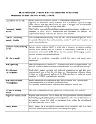
1. Shah Naseer (MS Comsats University Islamabad Abbottabad)
Difference between Different Velocity Models
Crustal velocity models Crustal seismic velocity models are used to locate earthquake hypocenters.
Typically, one dimensional velocity models are 3 - 8 fixed-thickness layers of varying P
and S velocities with depth. On occasion, the layers of the upper crust (0-2 kilometers)
are constrained with well log data from nearby wells
Community Velocity
Models
The CVMH is composed of detailed basin velocity descriptions that are based on tens of
thousands of direct velocity measurements and incorporate the locations and
displacements of major fault zones that influence basin structure
Unfiend Community
Velocity Models
The Unified Community Velocity Model (UCVM) software framework provides access
to detailed information about earth properties, namely P‐ and S‐wave velocities and
density, on regional scales
Seismic Velocity Modeling
(SVM)
Seismic velocity modeling (SVM) is a full suite of interactive applications enabling
velocity model building and the execution of depth-imaging workflows in a 3D
visualization environment. SVM delivers the most accurate depth-imaging solutions
currently available in an optimal timeframe.
3D velocity model Is based on a travel-time tomographic method from active- and passive-source
experiments
M-GS gridding M-GS gridding solutions consist of 3D kriging algorithms with varying parameters. They
take into account local structural characteristics of seismic velocities and their coverage.
3D calibration
(PSTM/PSDM
Used velocity models respecting both geological structuration and well data with a
minimum depth error far from the wells thanks to a 3D geostatistical calibration solution
is based on a 3D structural analysis of the differences between wells and seismic
velocities. In 3D M-GS bivariate kriging take place
M-GS surface model
(PSTM/PSDM)
Getting information the best prediction depth surfaces through these 4 possible steps
conditioning seismic velocities with geostatistical filters
3D calibration, depth conversion, calibration of the surfaces to the well tops
1D layered velocity
models
1D velocity-model building for application to microseismic data analysis.
Regional Velocity Models Regional and sub-regional velocity model by using geostatistical filtering algorithms,
factorial kriging, 3D gridding and a calibration performed. Also provide the estimation of
an uncertainty volume from which you can extract at any surface, the potential depth
error associated to the velocity model
Blocky Model Blocky models use a layer-based representation of the subsurface, each layer being
associated with a macrosequence in which the velocity varies gently

2. Name Type Sub Type Depth
Coverage
Areal
Coverage
Reference Earth Model also
known as REF (STW105)
1-D Reference Earth
Model
velocity model 0 to 6371.0 km Point data
Continental Parametric Earth Model (PEM-C) reflects different properties of the
continental upper mantle while Oceanic reflects different properties of the oceanic
upper mantle
1-D Reference Earth Model
(MEAN) or Ak135-f
1-D modified
IASP91 model
full model 0.0 - 6371.0 km spherical
average Earth
model
MEAN reference Earth model is based on the Earth model IASP91. MEAN
replaces IASP91’s mid-crustal discontinuity and Moho depth of 20 and 35 km to
18 and 30 km, respectively. It also replaces IASP91’s a high S-velocity zone of the
uppermost mantle (to the depth of 210 km) with a low S-velocity zone less than
4.5 km/s.
Iasp91 velocity model (Inactive) 1D Reference P and S velocities
0.0 - 6371.0 km
radial Earth
mode
A parameterised velocity model that has been constructed to be a summary of the
travel time characteristics of the main seismic phases.
A 1-D modified PEM-C S
velocity model (MC35)
1-D Reference Earth
Model
S velocity to 2885 km Continental
point data
MC35 reference Earth model is based on the continental Earth model PEM-C .
MC35 replaces PEM-C ‘s high- and low-velocity zones of the uppermost mantle
(to the depth of 210 km) with a constant shear-wave velocity of 4.5 km/s.
Smoothed Preliminary
Reference Earth Models
(SPREM)
1-D Reference Earth
Model
S velocity 40 to 680.0 km
Globa
PREM_Vsv and SPREM_Vsh reference Earth models are based on the global
reference model PREM with the discontinuities smoothed. For each propagation
path analyzed the crust of SPREM_Vsv or SPREM_Vsh is replaced by the path
averaged crust taken
Average of
the TNA and SNA models
1-D Reference Earth
Model
S velocity 0 to 2891 km Point data

3. (TNA/SNA) An average of the TNA (Tectonic North America) and SNA (Shield North
America) S velocity models of Grand and Helmberger (1984)
A 1-D modified PEM-C S
velocity model (MC35)
1-D Reference Earth
Model
S velocity 0 to 2885 km Continental
point data
MC35 reference Earth model is based on the continental Earth model PEM-C .
MC35 replaces PEM-C ‘s high- and low-velocity zones of the uppermost mantle
(to the depth of 210 km) with a constant shear-wave velocity of 4.5 km/s.
Global SV wave upper mantle
model updated until September
2017(3D2017_09Sv)
3-D Tomography
Earth Model
SV wave velocity,
Azimuthal
anisotropy and
peak to peak
anisotropy
40 to 1000 km Global
3D2017_09Sv is the current update of our background model 3D2015_07Sv up to
September 2017
3-D isotropic shear-wave model
for Africa from full-wave
ambient noise tomography
(Africa.ANT.Emry-etal.2018
3-D Tomography
Earth Model
Shear-wave
velocity (km/s)
Included in the
netCDF are depths
from 33-614 km;
best model
resolution is at
~100-400 km
(latitude: -41.4°
to 51.6°,
longitude: -32.6°
to 66.4°)
Africa.ANT.Emry-etal.2018 is a 3-D isotropic shear-wave tomographic model of
Africa and neighboring regions. Model is constrained by long period (40-340 sec.)
3D shear-wave velocity model
(Alaska.ANT+RF.Ward.2018)
3-D Tomography
Earth Model
Shear-wave
velocity (km/s)
0 to 70 km (bsl) The Alaskan
Cordillera
(latitude:
52°N/73°N,
longitude:
113°W/173W°)
The model incorporates seismic data from an earlier ambient noise tomography
study (Ward, 2015) along with new Transportable Array data to image the shear
wave velocity structure of the Alaskan Cordillera from the joint inversion of
surface wave dispersion and receiver functions.
Regional finite-frequency
teleseismic P-wave tomography
model for the Eastern
Mediterranean
3D Tomography
Earth Model
Relative P-wave
velocity (%dVp)
100.0 - 900.0 km Latitude: 26.0 to
49.0 Longitude:
12.0 to 57.0

4. Model uses relative arrival time residuals from 936 earthquakes recorded at 313
stations of a variety of temporary and permanent seismic deployments in Turkey,
Greece, Cyprus, and Armenia. Residuals are measured in four frequency bands and
inverted in a finite-frequency tomographic inversion
Preliminary Reference Earth
Model (PREM)
1-D Reference Earth
Model
full model 0 to 6371.0 km Point data
The Preliminary Reference Earth Model, Dziewonski and Anderson (1981) , is an
average Earth model that incorporates anelastic dispersion and anisotropy and
therefore it is frequency-dependent and transversely isotropic for the upper mantle.
Parametric Earth Models
(PEM)
1-D Reference Earth
Model
full model 0 to 6371.0 km Point data
Continental Parametric Earth Model (PEM-C) reflects different properties of the
continental upper mantle.s Oceanic Parametric Earth Model (PEM-O) reflects
different properties of the oceanic upper mantle
Global upper mantle surface
wave tomography
model(CAM2016)
3-D Tomography
Earth Model
S velocity Upper mantle (40
to 680 km
Global
CAM2016 is a group of global upper mantle models based on multi-mode surface
wave tomography
P- and S-velocity models for the
western US integrating body-
and surface-wave
constraints(DNA13)
3-D Tomography
Earth Model
P and S velocity
perturbations(%)
0 to 1280km (best
resolution 0 to
1000km)
United States
(25°/52°, -126°/-
72°)
The DNA13 model integrates teleseismic body-wave traveltime and surface-wave
phase velocity measurements into a single inversion to constrain the P- and S-wave
velocity structure s
A global compressional velocity
model of the mantle from
cluster Analysis of long-period
Waveforms (HMSL-P06)
3-D Tomography
Earth Model
Compressional
velocity
perturbation (%)
66 to 2900 km Global (-
90°/90°, -
180°/180°)
HMSL-P06 is an isotropic P velocity model with 18 layers (approximately 100 km
thickness in the upper mantle and 200 km in the lower mantle) and 2578 blocks in
each layer (approximately 4 degree equal area blocks at the equator). The upper
mantle is constrained to be a scaled
North American upper mantle
surface wave tomography model
(NA04)
3-D Tomography
Earth Model
S velocit Upper mantle (70
to 670 km)
North America
(10°/85°, -170°/-
55°)

5. NA04 is derived from inversion of the fundamental and higher mode Rayleigh
waveforms using the Partitioned Waveform Inversion technique, Nolet (1990) . The
data set used includes waveforms from about 1400 regional seismograms recorded
at North American digital broadband seismic stations (including the USArray
Transportable Array waveforms).
3D P-wave velocity model of
Yellowstone from joint inversion
of local earthquake and
teleseismic travel-time data(YS-P-
H15)
3-D Tomography
Earth Model
P-wave velocity
(km/s) and
perturbation (%)
-4 to 160 km (0
km refers to sea
level
Yellowstone
(latitude:
43.55°/45.2°,
longitude: -
111.55°/-
109.75°
The model integrates local earthquake and teleseismic travel-time data into one
inversion to constrain the 3-D P-wave velocity structures of Yellowstone from the
upper mantle to the upper crust
A global radially anisotropic
mantle shear velocity model with
improved crustal
corrections(SAW642ANb)
3-D Tomography
Earth Model
Anisotropic S
velocity
Whole Mantle
(~50 to ~2850 km)
Global (-
90°/90°, -
180°/180°)
SAW642ANb is a radially anisotropic shear velocity model, parameterized in terms
of isotropic S velocity (Voigt average) and the anisotropic parameter, xi
(Vsh2/Vsv2).

7. 3D

8. Alaska-S-SW-2018

9. ANA2_P_2018_

10. APVC
DNA

11. EAV

13. FWEA

14. DNA

15. PNW

16. LLNL

18. NA04

19. NA07

20. DNA13
NEUS

21. FWEA

22. NWUS11

26. SAW64

27. SAW64

28. SEM

29. Sglobe
SSs

30. STW

31. Taiwan