2. 22 2 Radiation of an Accelerated Charge
C
D
B
O
r
A
Δv t
Δv
Δv
t sinϑ
ϑ
Δt c
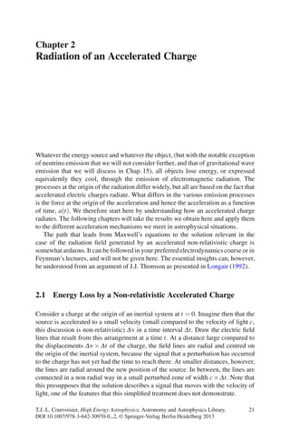
Fig. 2.1 Schematical view of the electric field lines at time t due to a charged particle accelerated
to a velocity Δv c in a time interval Δt (Adapted from Longair (1992))
Figure 2.1 gives the large picture and the detail of the perturbed field lines.
In this section we will denote electric fields by E in order to distinguish them
from the energy, denoted E. You can read from Fig. 2.1 that the ratio of the tangential
to the radial field line components in the perturbed zone is
Eθ
Er
=
Δv ·t sinθ
cΔt
. (2.1)
The radial field is given by the Coulomb law
Er =
e
r2
, e in e.s.u., r = ct. (2.2)
You can therefore deduce the tangential field component and find
Eθ = e·
Δv
Δt
sinθ
1
cr2
·t (2.3)
= e
¨rsinθ
c2r
. (2.4)
Note that this field depends on the distance to the centre as r−1 rather than r−2.
This is a characteristics of the radiation field in the far zone. The only electrical
field component that is relevant for radiation is that which is perpendicular to the
direction of propagation, i.e. Eθ . It is the one we consider further here.
3. 2.2 Spectrum of the Radiation 23
Introducing the electrical dipole moment p = e·r, we write
Eθ =
¨psinθ
c2r
. (2.5)
We may now calculate the energy flux carried by this disturbance. The energy
flux transported by electromagnet fields is given by the Poynting vector S:
S =
c
4π
E× B. (2.6)
The magnetic field is equal and perpendicular to the electric field in electromag-
netic radiation:
B = n× E (2.7)
Using (2.5) the energy loss in the direction θ in a solid angle dΩ, dE
dt dΩ =
|S|r2 dΩ, is therefore
dE
dt
dΩ =
c
4π
| ¨p|2 sin2
θ
c4r2
·r2
dΩ. (2.8)
In order to find the energy loss from the charge, one needs to integrate (2.8)
over the solid angle dΩ. The configuration is cylindrically symmetrical around the
direction of the acceleration. The integration over one angle is therefore trivial and
dΩ = 2π sinθdθ. The result is
dE
dt
=
c
4π
| ¨p|2
c4
π
0
2π sin3
θ dθ =
2
3
| ¨p|2
c3
(2.9)
This is the so-called Larmor formula. It is given here in Gaussian units and gives
the energy carried by the electromagnetic radiation emitted by an accelerated charge
as a function of this acceleration. The radiation is dipolar (see the sin2
θ in (2.8)).
The absolute value is there to remind us that the sign will be different whether one
considers the energy loss from the charge or the gain in the radiation.
2.2 Spectrum of the Radiation
One may use the results we have obtained for the energy radiated by an accelerated
charge to calculate the spectrum of the emitted radiation. This is done by considering
the Fourier transform of the dipole, and calculating from there that of the electric
field and of the energy flux. The Fourier transform of the dipole p(t) is given by
p(t) =
∞
−∞
e−iωt
ˆp(ω)dω. (2.10)
Remember that the Fourier transform of the second time derivative of a function
is given by
4. 24 2 Radiation of an Accelerated Charge
¨p(t) = −
∞
−∞
ω2
e−iωt
ˆp(ω)dω. (2.11)
Writing the definition of the transform of the electric field on one side and taking
the Fourier transform of (2.5) on the other side, one obtains using (2.11)
Eθ (t) =
∞
−∞
e−iωt ˆE (ω)dω (2.12)
= −
∞
−∞
ω2
e−iωt
ˆp(ω)
sinθ
c2r
dω, (2.13)
from which we read the following expression for the Fourier transform of the
electric field
ˆE (ω) = −ω2
ˆp(ω)
sinθ
c2r
. (2.14)
Integrating the energy loss (2.9) over time one finds the energy that crosses a
surface per surface element dA
dE
dA
=
∞
−∞
energy flux·dt =
∞
−∞
c
4π
E 2
(t)dt (2.15)
where we have used the fact that the energy flux is given by the Poynting
vector (2.6).
From the theory of Fourier transforms we use
∞
−∞
E 2
(t)dt = 2π
∞
−∞
| ˆE (ω)|2
dω = 4π
∞
0
| ˆE (ω)|2
dω (2.16)
and therefore
dE
dA
= c
∞
0
| ˆE (ω)|2
dω (2.17)
giving finally the emitted spectrum
dE
dω
= c| ˆE (ω)|2
dA (2.18)
(2.14)
== c
ω4| ˆp(ω)sinθ|2
c4r2
dA (2.19)
=
8π
3
ω4
c3
| ˆp(ω)|2
(2.20)
This shows that in a non-relativistic approximation (remember that we assumed
Δv to be small compared to the velocity of light) the spectrum is proportional to the
square of the Fourier transform of the dipole moment.
5. 2.3 Radiation of a Relativistic Accelerated Particle 25
2.3 Radiation of a Relativistic Accelerated Particle
Not all the radiating charges that we will meet in this book are non-relativistic. We
will see that, often, very high energy particles must be present in order to explain
the observed radiation. It is therefore also necessary to know how relativistically-
moving charges radiate. In order to approach this question we introduce the basic
elements of special relativity, which we will use whenever appropriate. We do not
give a presentation of special relativity here, rather, we recall those elements that we
need for the derivation. We will introduce further elements as they become necessary
in the following chapters.
In special relativity one considers the flat metric of four-dimensional space time
ds2
= c2
dτ2
= c2
dt2
− dx2
, (2.21)
which describes the distance between two events in space time. This distance is
invariant under the Lorentz transformations
t = γ t −
v
c2
x ,x = γ(x− vt),y = y,z = z, (2.22)
where γ = 1 − β2
−1
is the usual gamma factor, β = v
c , and v is the relative velocity
of the reference frames along the x-axis.
We next introduce the four-velocity
uμ
=
dxμ
dτ
, (2.23)
which, as a small difference between coordinates, is a vector. Written explicitly
u0
=
dx0
dτ
= c
dt
dτ
= γ ·c, (2.24)
because
(
dτ
dt
)2
= (dt2
−
1
c2
dx2
)/dt2
= 1 −
v2
c2
=
1
γ2
. (2.25)
Similarly
u =
dx
dτ
= γ ·v, (2.26)
as
(
dτ
dx
)2
= (dt2
−
1
c2
dx2
)/dx2
= (
1
v2
−
1
c2
)ev =
1
v2
1
γ2
ev, (2.27)
where ev is a unit vector in the direction of the velocity. Note that we will write v to
mean three-velocity, and in general bold italics vectors are three dimensional while
bold upright vectors are four dimensional.
6. 26 2 Radiation of an Accelerated Charge
The acceleration is the second proper time derivative of the coordinates
aμ
=
duμ
dτ
, (2.28)
which from (2.24) and (2.26) gives
a0
= c·
dγ
dτ
(2.29)
ai
=
d(γ ·vi)
dτ
. (2.30)
In order to generalise these results to describe the radiation of a non-relativistic
accelerated charge to relativistic charges, we write (2.9) in an explicitly covariant
form, i.e. in a form that is explicitly invariant under Lorentz transformations. In the
system in which the particle is at rest, we have
γ = 1,dτ = dt ⇒ a0
= 0,ai
=
dvi
dt
. (2.31)
In this system, the non-relativistic derivation of Sect. 2.1 is valid, and we know
that the energy carried by the radiation field created by an accelerated charge per
unit time P = dE
dt is
P =
2
3
e2 |˙v|2
c3
=
2
3
e2
c3
a·a, (2.32)
where a · a is the scalar product of the four-vector a with itself. To obtain the last
equality in Eq. 2.32, we have used Eqs. 2.28–2.31. The formulation
P =
2
3
e2
c3
a·a (2.33)
is manifestly covariant. In order to convince yourself of this, consider the transfor-
mations of the left part of the equality under Lorentz transformations
Energy → γ ·Energy (2.34)
Δt → γ ·Δt (2.35)
therefore
dE
dt
→
dE
dt
. (2.36)
This is clearly a scalar. The right side of the equality is a scalar product and thus
also a scalar. The equality (2.33) is therefore valid in all systems of reference and
corresponds to the relativistic generalisation of the Larmor formula (2.9) that we
were seeking.
7. 2.4 Relativistic Aberration 27
We can now write Eq. 2.33 in the system of the observer in which the particle is
moving relativistically explicitly as
P =
2
3
e2
c3
c2 dγ
dτ
2
−
d(γ ·v)
dτ
2
(2.37)
Doing the algebra and using
dγ
dτ
=
γ3
c2
v·
dv
dτ
, (2.38)
one obtains
P =
2e2
3c3
γ6
− ˙v·
v
c
2
−
|˙v|2
γ2
(2.39)
and
|P| =
2e2
3c3
γ6
a2
+
1
γ2
a2
⊥ , (2.40)
where we have introduced (v · ˙v) = v · a and |v × ˙v| = v · a⊥, the components of
the acceleration parallel and perpendicular to the velocity, and where we have used
|˙v|2 = a2 +a2
⊥. The sign is naturally different if one considers the energy lost by the
particles or that gained by the radiation field, and must be set accordingly. The power
radiated by a relativistically-moving accelerated charge is finally expressed as
P =
2e2
3c3
γ4
(a2
⊥ + γ2
a2
). (2.41)
2.4 Relativistic Aberration
In order to understand the properties of the light observed from a relativistically-
moving source it is still necessary to see how the geometry of the emission differs
between the rest frame of the charge and that of the observer. Consider a source
moving with a velocity v along the x-axis with respect to an observer and write with
“ ” the coordinate system in which the source is at rest, the “source system” in the
following. Both systems are related by the Lorentz transformation
x = γ(x− vt)
y = y
z = z
t = γ t − v
c2 x
(2.42)
8. 28 2 Radiation of an Accelerated Charge
photon: u'y = c
e− at rest
observer: vx = −v
x'
y'
x
y
1/γ
Fig. 2.2 The source at rest in
the primed system of
reference emits a photon
along the y-axis,
perpendicular to the velocity
of the observer who sees the
photon with an angle of
90◦ −1/γ from the observer’s
y axis
Consider now a photon emitted by the source along a direction, say the y -axis,
perpendicular to the velocity v. The photon moves with the speed of light: uy = c,
while all other components vanish in the source rest frame, see Fig. 2.2.
The transformation of the velocities is given by
ux =
dx
dt
=
γ(dx + vdt )
γdt (1 + v
c2 ux)
=
ux + v
1 + vux
c2
(2.43)
uy =
dy
dt
=
dy
γdt (1 + v
c2 ux)
=
uy
γ(1 +
vux
c2 )
(2.44)
uz =
dz
dt
=
dz
γdt (1 + v
c2 ux)
=
uz
γ(1 +
vux
c2 )
(2.45)
which for the special case of our photon simplifies to ux = v, uy = c
γ and uz = 0.
Consider now the direction under which the photon is observed in the observer’s
restframe
tanθ =
uy
ux
=
1
γβ
, (2.46)
where, as usual β = v
c .
We conclude from this analysis that all the photons emitted by a moving source
in the forward half sphere are observed as coming from a cone of half opening angle
(γβ)−1
in the observer’s rest frame. The change of apparent direction under which
the photon is observed in both frames is called the relativistic aberration. The fact
that all the photons emitted in a half sphere appear in a small cone leads to what
is called beaming. The source appears much brighter to observers lying within the
cone than to those located outside the cone.
We now have the tools needed to understand the radiation emitted by charges
accelerated through different forces. In the following chapters we will deduce
the properties of the radiation emitted by the different processes by estimating or
calculating the second derivative of the dipole moment and deducing the efficiency
9. References 29
of the process through the energy-loss formula of Larmor (2.9) or its relativistic
generalisation (2.41) using beaming where appropriate (2.46). The source spectra
will be calculated using Eq. (2.20).
2.5 Bibliography
Detailed derivations of the results presented here can be found in Jackson (1975)
for the classical electrodynamics and in Rybicki and Lightman, (2004) and Longair
(1992).
References
Jackson J.D., 1975, Classical Electrodynamics, second edition, John Wiley and Sons Inc.
Rybicki G.B. and Lightman A.P., 2004, Radiative Processes in Astrophysics, Wiley-VCH Verlag
Longair M. S., 1992, High Energy Astrophysics 2nd edition volume 1, Cambridge University Press