Chapter 1
Recollections from Elementary Quantum
Physics
Abstract We recall the prerequisites that we assume the reader to be familiar with,
namely the Schrödinger equation in its time dependent and time independent form,
the uncertainty relations, and the basic properties of angular momentum.
Introductory courses on quantum physics discuss the one-dimensional Schrödinger
equation for the wave function Ψ (x,t) of a particle of mass M moving in a poten-
tial V
i
∂Ψ
∂t
= −
2
2M
∂2Ψ
∂x2
+ V Ψ. (1.1)
Therein = h/2π is the reduced Planck constant. The function Ψ is understood as a
probability amplitude whose absolute square |Ψ (x,t)|2 = Ψ ∗(x,t)Ψ (x,t) gives the
probability density for finding the particle at time t at position x. This probability
density is insensitive to a phase factor eiϕ. With the Hamilton operator
H = −
2
2M
∂2
∂x2
+ V, (1.2)
the Schrödinger equation reads
˙Ψ = −
i
HΨ. (1.3)
The dot denotes the time derivative.
In this text, we print operators and matrices in nonitalic type, like H, p, or σ, just
to remind the reader that a simple letter may represent a mathematical object more
complicated than a number or a function. Ordinary vectors in three-dimensional
space are written in bold italic type, like x or B.
The time dependent Schrödinger equation reminds us of the law of energy con-
servation E = p2/2M + V if we associate the operator i ∂/∂t with energy E and
the operator ( /i)∂/∂x with momentum p. Take as an example the plane wave
Ψ (x,t) = Ψ0ei(kx−ωt) of a photon propagating in the x-direction. The energy opera-
tion i ∂Ψ/∂t = ωΨ then relates energy to frequency, E = ω, and the momentum
operation ( /i)∂Ψ/∂x = kΨ relates momentum to wave number, p = k.
D. Dubbers, H.-J. Stöckmann, Quantum Physics: The Bottom-Up Approach,
Graduate Texts in Physics,
DOI 10.1007/978-3-642-31060-7_1, © Springer-Verlag Berlin Heidelberg 2013
3

4 1 Recollections from Elementary Quantum Physics
The probability amplitude Ψ (x,t) for finding the particle at time t at position x
and the amplitude Φ(p,E) for finding it with energy E and momentum p turn out
to be Fourier transforms of each other. Pairs of Fourier transforms have widths that
are reciprocal to each other. If the width x in position is large, the width p in
momentum is small, and vice versa, and the same for the widths t and E. The
conjugate observables p and x or E and t obey the uncertainty relations
p x ≥
1
2
, E t ≥
1
2
. (1.4)
The exact meaning of x, etc. will be defined in Sect. 3.4.
For stationary, that is, time independent potentials V (x), the Hamilton operator
(1.2) acts only on the position variable x. The solution of the Schrödinger equation
then is separable in x and t,
Ψ (x,t) = ψ(x)e−iEt/
. (1.5)
The probability density (in units of m−1) for finding a particle at position x then is
independent of time |Ψ (x,t)|2 = |ψ(x)|2. The amplitude ψ(x) is a solution of the
time independent Schrödinger equation
−
2
2M
∂2ψ(x)
∂x2
+ V (x)ψ(x) = Eψ(x). (1.6)
In operator notation, this reads
Hψ = Eψ. (1.7)
For particles trapped in a potential well V (x), the requirement that total proba-
bility is normalizable to
+∞
−∞
ψ(x)
2
dx = 1 (1.8)
leads to the quantization of energy E such that only a discrete set of values En, with
the corresponding wave functions ψn(x), n = 1,2,3,..., is allowed. n is called the
main quantum number.
The mean value derived from repeated measurements of a physical quantity or
observable A is given by its expectation value
A(t) =
+∞
−∞
Ψ ∗
(x,t)AΨ (x,t)dx. (1.9)
For a stationary state Eq. (1.5), the expectation value A does not depend on time
and is insensitive to any phase factor eiϕ. For example, the mean position x of a
matter wave is given by the weighted average
x =
+∞
−∞
x ψ(x)
2
dx. (1.10)

1 Recollections from Elementary Quantum Physics 5
Sometimes the Hamiltonian H can be divided into two parts H = H1(x)+H2(y),
one depending on one set of (not necessarily spatial) variables x, the other on a
disjoint set of variables y. Then, as shown in standard textbooks, the solution of
the Schrödinger equation is separable in x and y as ψ(x,y) = ψ1(x)ψ2(y). As in
Eq. (1.5), we must attach a phase factor to obtain the time dependent solution
Ψ (x,y,t) = ψ1(x)ψ2(y)e−iEt/
. (1.11)
The probability densities for the joint occurrence of variable x and variable y then
multiply to
Ψ (x,y,t)
2
= ψ1(x)
2
ψ2(y)
2
. (1.12)
This is consistent with classical probability theory, where probabilities multiply for
independent events. The probability that two dice both show 5 is 1
6 × 1
6 = 1
36 .
If, on the other hand, the quantum system can evolve along two mutually exclu-
sive paths ψ1 or ψ2, as is the case in the famous double-slit experiments, then the
two probability amplitudes add coherently, and the total probability is
|Ψ |2
= |ψ1 + ψ2|2
= |ψ1|2
+ |ψ2|2
+ 2|ψ1||ψ2|sinδ, (1.13)
with phase angle δ. Only if phase coherence between the partial waves ψ1 and ψ2
is lost, does the total probability equal the classical result
|Ψ |2
= |ψ1|2
+ |ψ2|2
, (1.14)
with probabilities adding for mutually exclusive events. The probability that a die
shows either 5 or 3 is 1
6 + 1
6 = 1
3 .
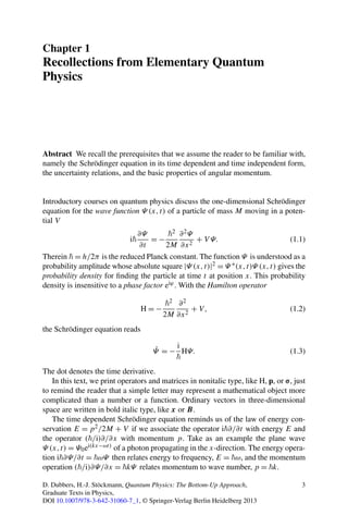
Figure 1.1 shows the setup and result of a double-slit experiment with a beam of
slow neutrons. What we see is the self-interference of the probability amplitudes ψ1
and ψ2 of single neutrons. The conditions for the appearance of quantum interfer-
ence will be discussed in Sect. 6.6.
For most students the Schrödinger equation is no more difficult than the many
other differential equations encountered in mechanics, electrodynamics, or trans-
port theory. Therefore, students usually have fewer problems with the ordinary
Schrödinger equation than with a presentation of quantum mechanics in the form
of matrix mechanics. In everyday scientific life, however, spectroscopic problems
that require matrix diagonalization are more frequent than problems like particle
waves encountering step potentials and other scattering problems. Furthermore, as
we shall see in Sect. 19.1.2, the Schrödinger equation can always equally well be ex-
pressed as a matrix equation. Therefore, matrix mechanics is the main topic of the
present tutorial. Instead of starting with the Schrödinger equation, we could have
started with the Heisenberg equation of motion (discovered a few weeks before the
Schrödinger equation) because both are equivalent. We postpone the introduction
of Heisenberg’s equation to Chap. 10 because students are less familiar with this
approach.

6 1 Recollections from Elementary Quantum Physics
Fig. 1.1 (a) Double-slit experiment with neutrons: The monochromatic beam (along the arrow),
of de Broglie wave length λ = 2 nm, λ/λ = 8 %, meets two slits, formed by a beryllium wire
(shaded circle) and two neutron absorbing glass edges (vertical hatching), installed on an optical
bench of 10 m length with 20 µm wide entrance and exit slits. (b) The measured neutron self-in-
terference pattern follows theoretical expectation. From Zeilinger et al. (1988)
To begin we further assume acquaintance with some basic statements of quantum
physics that are both revolutionary and demanding, and our hope is that the reader
of this text will learn how to live and work with them. The first statement is: To any
physical observable A corresponds an operator A. The measurement of the observ-
able A leaves the system under study in one of the eigenstates or eigenfunctions ψn
of this operator such that
Aψn = anψn. (1.15)
The possible outcomes of the measurement are limited to the eigenvalues an. Which
of these eigenfunctions and eigenvalues is singled out by the measurement is uncer-
tain until the measurement is actually done.
If we regard the ordered list ψn as elements of a vector space, called the Hilbert
space, the operation A just stretches an eigenvector ψn of this space by a factor an.
The best-known example of an eigenvalue equation of this type is the time indepen-
dent Schrödinger equation
Hψn = Enψn. (1.16)
H is the operator for the observable energy E, ψn are the eigenfunctions of energy,
and En are the corresponding eigenvalues. In this text, we shall only treat the sim-
plest case where the spectrum of the En is discrete and enumerable, as are atomic
energy spectra, and in most cases limit the number of energy levels to two.
Another basic statement is derived in Sect. 3.4: Two physical quantities, de-
scribed by operators A and B, can assume well defined values an and bn, simultane-
ously measurable with arbitrarily high precision and unhampered by any uncertainty
relation, if and only if they share a common set of eigenfunctions ψn, with
Aψn = anψn, Bψn = bnψn. (1.17)

1 Recollections from Elementary Quantum Physics 7
An important operator is that of the angular momentum J, which we shall de-
rive from first principles in Chap. 16. Let us beforehand recapitulate the following
properties of J, as known from introductory quantum physics. The components Jx,
Jy, and Jz of the angular momentum operator J cannot be measured simultaneously
to arbitrary precision. Only the square magnitude J2 of the angular momentum and
its component Jz along an arbitrary axis z are well defined and can be measured
simultaneously without uncertainty. This means that the phase of J about this axis
z remains uncertain. The operators of the two observables J2 and Jz then must have
simultaneous eigenfunctions that we call ψjm, which obey
J2
ψjm = j(j + 1) 2
ψjm, (1.18a)
Jzψjm = m ψjm, (1.18b)
with eigenvalues j(j + 1) 2 and m , respectively.
Angular momentum is quantized, with possible angular momentum quantum
numbers j = 0, 1
2 ,1, 3
2 ,.... For a given value of j, the magnetic quantum number
m can take on only the 2j + 1 different values m = −j,−j + 1,...,j.
For j = 1
2 we have m = ±1
2 and
J2
ψ1
2 ,± 1
2
=
3
4
2
ψ1
2 ,± 1
2
, (1.19a)
Jzψ1
2 ,± 1
2
= ±
1
2
ψ1
2 ,± 1
2
. (1.19b)
If we arrange the 2j + 1 eigenfunctions of the angular momentum ψjm into one
column
ψj =
⎛
⎜
⎜
⎜
⎝
ψj,j
ψj,j−1
...
ψj,−j
⎞
⎟
⎟
⎟
⎠
, (1.20)
we shall print this column vector ψj in nonitalic type, as we did for the operators.
The corresponding row vector is ψ†
j = (ψ∗
j,j ,ψ∗
j,j−1,...,ψ∗
j,−j ), where the dagger
signifies the conjugate transpose ψ† = ψ∗T of a complex vector (or matrix).
The components Jx and Jy of the angular momentum operator J do not have
simultaneous eigenfunctions with J2 and Jz. If we form the linear combinations
J+ = Jx + iJy, J− = Jx − iJy, (1.21)
these operators are found to act on the angular momentum state ψjm as
J+ψjm = j(j + 1) − m(m + 1)ψj,m+1, (1.22a)
J−ψjm = j(j + 1) − m(m − 1)ψj,m−1, (1.22b)

8 1 Recollections from Elementary Quantum Physics
with J+ψj,+j = 0 and J−ψj,−j = 0. The J+ and J− are the raising and lowering
operators, respectively. For j = 1
2 we have J+ψ1
2 ,− 1
2
= ψ1
2 ,+ 1
2
and J−ψ1
2 ,+ 1
2
=
ψ1
2 ,− 1
2
.
Angular momentum may be composed of the orbital angular momentum L and
of spin angular momentum S, which can be added to the total angular momentum
J = L + S. The orbital angular momentum quantum number l can only have integer
values, spin quantum number s can have either integer or half-integer values. The
triangle rule of vector addition tells us that the (integer or half-integer) angular
momentum quantum number j has the allowed range
|l − s| ≤ j ≤ l + s. (1.23)
The total angular momentum quantum number is
m = ml + ms, (1.24)
going in unit steps from m = −j to m = j. For example, two angular momenta with
l = 1 and s = 1
2 can be added to j = 1
2 or j = 3
2 . For l = 0, j = s we have m = ms,
and for s = 0, j = l we have m = ml. For the sake of simplicity, in these two special
cases we shall always write m for the respective magnetic quantum numbers ms
or ml.
References
Zeilinger, A., Gähler, R., Shull, C.G., Treimer, W., Mampe, W.: Single- and double-slit diffraction
of neutrons. Rev. Mod. Phys. 60, 1067–1073 (1988)

http://www.springer.com/978-3-642-31059-1