explains the formation of frequency distribution table

2. •Frequency Distribution Table
Data
Frequency
Class
Class interval
Range
Frequency Distribution Table

3. •Statistics– Definition
Statistics is a branch
of Mathematics. It
collects, enumerate,
organize, tabulates,
calculates, interprets
the data and gives the
results.
The science of average is
statistics (Prof. Bowley).

4. •Statistics– Definition
It’s all perfectly clear;
you compute statistics
from statistics by
statistics. (Tate, 1955)
It’s all perfectly clear; you
compute statistics (M, Me, Mo)
from statistics (Data) by
statistics (formula).
Data – Plural
Datum - Singular

5. •Organization of Data
✓ Data speaks.
✓ To understand it, it has to
organized.
✓ One form of organization is
Frequency Distribution
Table

6. •Frequency Distribution Table - Definition
✓ If the frequency of each
classes which was formed
from data are listed in a
form of a table called as
Frequency Distribution
Table.

7. •Frequency Distribution Table - Steps
1. Arrange the data in increasing order
2. Find range (R)
3. Determine the number of classes
4. Form frequency distribution table

8. •1. Arrange the data in increasing order
•(N=56, Where N is total number of data )
42, 43, 60, 61, 77, 79, 78,
50, 53, 60, 63, 78, 77, 52,
53, 64, 60, 76, 68, 69, 54,
91, 62, 92, 88, 63, 74, 86,
71, 70, 80, 59, 77, 65, 67,
80, 83, 71, 73, 82, 56, 72,
65, 57, 55, 65, 69, 58, 56,
67, 67, 56, 75, 68, 68, 62
Raw Data
42, 43, 50, 52, 53, 53, 54, 55,
56, 56, 56, 57, 58, 59, 60, 60,
60, 61, 62, 62, 63, 63, 64, 65,
65, 65, 67, 67, 67, 68, 68, 68,
69, 69, 70, 71, 71, 72, 73, 74,
75, 76, 77, 77, 77, 78, 78, 79,
80, 80, 82, 83, 86, 88, 91, 92
Arranged in ascending order

9. •2. Find Range (R)
42, 43, 50, 52, 53, 53, 54, 55,
56, 56, 56, 57, 58, 59, 60, 60,
60, 61, 62, 62, 63, 63, 64, 65,
65, 65, 67, 67, 67, 68, 68, 68,
69, 69, 70, 71, 71, 72, 73, 74,
75, 76, 77, 77, 77, 78, 78, 79,
80, 80, 82, 83, 86, 88, 91, 92
Range = Highest Score –
Lowest Score
= 92 – 42
= 50

10. •Class - Concept
If the data are grouped
within a boundary, they are
called as the classes.
(1-5), (6-10), (11-15) ….. are
called as classes. Another
example for class could be
(1-10), (11-20), (21-30),….
Each class will be having
upper limit and lower
limit. For example for the
class (1-10), the
Upper limit is 10 and
Lower limit is 1
The data
1,2,3,4,5,6,7,8,9,10
belongs to this class

11. •Class - Concept
The class (1-10) can be
represented as
Let us take the case of 1.
it can be represented as
The range of 1 starts from
0.5 to 1.5. The data .5, .6,
.7, .8, .9, 1, 1.1, 1.2, 1.3,
1.4, 1.5 belongs to 1

12. •Class Interval (i) - Concept
Hence, the real lower limit is
0.5 instead of 1 and the real
upper limit is 10.5 instead of
10. Consider the case of 10
Class interval
= Real Upper limit – Real
lower limit
= 10.5 – 0.5
= 10
Class interval is the
distance between the real
upper and lower limits.

13. •3. Determine the number of classes
Number of classes
= R/i
= 50 / 5
= 10
= 10 + 1
= 11
(Always 1 has to
be added, so
eleven classes)
There are three variables; No. of
classes, Range (R), and class interval
(i). To find number of classes, R and i
should be known. R is 50. i has to
fixed logically.
For better statistical calculation 8 to
15 classes are necessary. So, if one
has to have 8 to 15 classes, i can be
fixed as 5. If you keep i as 10, only 6
classes would be formed.

14. Classes
Since 11 classes is
the answer. First
class is formed
which includes the
lowest number 42.
The class is 40-44.
By keep on adding
the classes the last
class would be 90-
94
40 - 44, 45 - 49, 50 - 54, 55 - 59,
60 - 64, 65 - 69, 70 - 74, 75 - 79,
80 - 84, 85 - 89, 90 - 94
Classes

15. •Frequency Distribution Table - Definition
✓ If the frequency of each
classes which was formed
from data are listed in a
form of a table called as
Frequency Distribution
Table.

16. 4. Form Frequency Distribution Table
Data which has been made into
ascending order is on the left. Classes
that has been formed in the previous
slide. Have the classes as the column I.
Then for each class find the number of
incumbents. For example data 42 and
43 fits in the class 40-44. This can be
made as Tally. Tally marks forms the
column II. The third column gives the
total number of tallies which is
frequency (f). Column I,II and III forms
the frequency distribution table.
42, 43, 50, 52, 53, 53,
54, 55, 56, 56, 56, 57,
58, 59, 60, 60, 60, 61,
62, 62, 63, 63, 64, 65,
65, 65, 67, 67, 67, 68,
68, 68, 69, 69, 70, 71,
71, 72, 73, 74, 75, 76,
77, 77, 77, 78, 78, 79,
80, 80, 82, 83, 86, 88,
91, 92

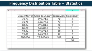
17. 4. Form Frequency Distribution Table
42, 43, 50, 52, 53, 53, 54,
55, 56, 56, 56, 57, 58, 59,
60, 60, 60, 61, 62, 62, 63,
63, 64, 65, 65, 65, 67, 67,
67, 68, 68, 68, 69, 69, 70,
71, 71, 72, 73, 74, 75, 76,
77, 77, 77, 78, 78, 79, 80,
80, 82, 83, 86, 88, 91, 92

18. Assignment
Have around 60 hypothetical data and form
frequency distribution table.

19. References
• Garrett, H. E. (1926). Statistics in psychology and education. New York: Longman’s
Green & Co
• Mathew, T.K., and Mollykutty, T.M. (2011). Science education -Theoretical bases of
teaching and pedagogic analysis - Physical Science and Natural Science. Kerala:
Rainbow Book Publishers
• Mangal. S. K. (2014). Statistics in psychology and education. Delhi: PHI Learning Private
Limited
• NCERT. (2013). Teaching of science. Delhi: Author
• Radha Mohan. (2007). Teaching of physical science. (3rd ed.). Delhi: PHI Learning
• Rathinasabapathy, P. (2001). கல்வியில் தேர்வு [Examination in Education]. (2nd
ed.). Chennai: Shantha Publishers.
• Srinivasan, P. (2011). அறிவியல் கற்பிே்ேல் [Teaching of science]. Thanjavur: DDE,
Tamil Univeristy
• Images from google