Seismic

1. Introduction to Seismology: Lecture Notes
16 March 2005
TODAY’S LECTURE
1. Snell’s law in spherical media
2. Ray equation
3. Radius of curvature
4. Amplitude → Geometrical spreading
5. τ – p
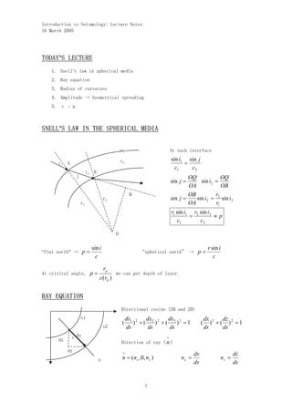
SNELL’S LAW IN THE SPHERICAL MEDIA
c1 At each interface
c2 sin i1 sin j
i1 A =
c1 c2
i2 B
j OQ OQ
sin j = sin i2 =
OA OB
Q OB r
r2 sin j = sin i2 = 2 sin i2
r1 OA r1
r1 sin i1 r2 sin i2
= ≡p
c1 c2
O
sin i r sin i
“flat earth” → p= “spherical earth” → p=
c c
rp
At critical angle, p= we can get depth of layer.
c(rp )
RAY EQUATION
Directional cosine (3D and 2D)
s1 dx1 2 dx dx dx 2 dz
( ) + ( 2 )2 + ( 3 )2 = 1 ( ) + ( )2 = 1
s2 ds ds ds ds ds
dz i ds ∧
Direction of ray ( n )
dx ∧ dx dz
n n = (n x ,0, n z ) nx = nz =
ds ds
1

2. Introduction to Seismology: Lecture Notes
16 March 2005
1∧
Using Eikonal equation ∇T = n,
c
Generalized Snell’s law (Ray Equation)
d 1 d 1 dxi
( )= ( )
dxi c( x) ds c( x) ds
This equation means that the change of wavespeed is related to change of ray geometry.
If there is no change in x direction, the derivative of x direction should be zero.
d 1 dx 1 dx sin i
( )=0 ⇒ = Const. ⇒ = Const. ⇒ Snell’s law !!
ds c(x) ds c ds C
How does this angle i change in the direction of propagation?
d di dz di d di ( s ) dc
(sin i) = cos i = = ( pc) ⇒ =p
ds ds ds ds ds ds dz
Therefore, the change of angle is related to the change of velocity.
dc di
If is large ⇒ is large
dz ds
dc di
If is zero (c = const.) ⇒ is zero (i = const.) Straight
dz ds
Ray !!
RADIUS OF CURVATURE
R : the radius of curvature
ds = Rdi
ds 1 dz 1 1
R= = = ⇒ R=
di di p dc dc dc
p( ) p( )
dz dz
R
R is related to wavespeed gradient and ray parameter.
dz i ds
dc
dx If =0 ⇒R → ∞ Straight Ray !!
dz
2

3. Introduction to Seismology: Lecture Notes
16 March 2005
dc
If large ⇒ rapid change in c Strong Gradient
dz
r sin i
from p = ,
c
small i → small p → large R
i
AMPLITUDE-GEOMETRICAL SPREADING
Focusing-defocusing
Shadow Zone
Focusing effect Defocusing effect
We examine the property of dp / dx
dp d dT d 2T
= ( )= 2
dx dx dx dx
Small dx and large dp → dp / dx goes to infinity → large amplitude (focusing)
Large dx and small dp → dp / dx goes to zero → small amplitude (Shadow zone)
We also examine x( p )
x
ds x/2
T =2 tan i =
i c h
c ds
h
3

4. Introduction to Seismology: Lecture Notes
16 March 2005
One layer : x = 2h tan i
n
Multiple layers : x =
2 ∑h
j =0
j tan i j
Continuous case
zp zp zp zp
1 dz dz
x( p ) =
2 ∫ tan idz =
2
p ∫
( −
p 2 )
−1/ 2 dz =
2
p ∫
=
2 p ∫
0 0 c( z )
2
0 1 / c 2 −
p 2 0
η
d ⎧ ⎫ dx ⎧ ⎫ ⎧ p d 2c ⎫
zp zp z
dx dz ⎪ dz ⎪ 1 ⎪ ⎪
= 2 ∫
+ 2 p ⎨
∫
⎬
⇒
≈ ⎨− ⎬ + ⎨+ ∫ 2 dz ⎬
dp 2
1 / c −
p 2 2 2
dp ⎪ 0 1 /
c − p ⎪ dp ⎩ (dc / dz ) 0 ⎭ ⎪ 0 dz
⎩ ⎪
⎭
0 ⎩ ⎭
The change of distance in terms of ray parameter is related to gradient of wave speed
at surface and gradient of the change in wavespeed between surface and turning point.
d 2c
Changes of velocity gradient, , are small → large distance x for smaller ray
dz 2
dx
parameter p, < 0 → “Normal” or Prograde behavior
dp
T
c(z)
dx
<0
z
dp
Δ
4

5. Introduction to Seismology: Lecture Notes
16 March 2005
Distance (�)
Intercept time (�)
Depth
Velocity Ray parameter (p)
Ray parameter (p)
Time
Distance (�) Distance (�)
Figure by MIT OCW.
This figure represents ray paths, T ( ∆ ) , p( ∆ ) , and τ ( p) relationships for
velocity increasing slowly with depth.
( Adapted from S. Stein and M. Wysession (2003), An Introduction to Seismology, Earthquakes,
and Earth Sturcture, Blackwell Publishing, p160)
5

6. Introduction to Seismology: Lecture Notes
16 March 2005
d 2c
Changes of v elocity gradient, , are large → samll distance x for smaller ray
dz 2
dx
parameter p, > 0 → Retrograde behavior
dp
dx
If dp ≠ 0 and dx = 0 → = 0 → “Caustic” or focusing effect
dp
c(z)
z
dx
Caustic, dp = 0 large amplitude
dx
>0
dp dx
<0
dp
dx
<0
dp
6

7. Introduction to Seismology: Lecture Notes
16 March 2005
Distance (�)
Intercept time (�)
Depth
Velocity Ray parameter (p)
Ray parameter (p)
Time
Distance (�) Distance (�)
Figure by MIT OCW.
This figure represents ray paths, T ( ∆ ) , p( ∆ ) , and τ ( p) relationships for velocity
increasing rapidly with depth. In this case we can see the triplication and retrograde
behavior.
( Adapted from S. Stein and M. Wysession (2003), An Introduction to Seismology,
Earthquakes, and Earth Sturcture, Blackwell Publishing, p160)
7

8. Introduction to Seismology: Lecture Notes
16 March 2005
Distance (�)
Intercept time (�)
Depth
Velocity Ray parameter (p)
Ray parameter (p)
Time
Distance (�) Distance (�)
Figure by MIT OCW.
This figure represents ray paths, T ( ∆ ) , p( ∆ ) , and τ ( p) relationships for velocity
decreasing slowly within a low-velocity zone. In this case we can see the shadow zone
where no direct geometric arrivals appear, and hence discontinuous T ( ∆ ) , p( ∆ ) , and τ ( p) curves.
( Adapted from S. Stein and M. Wysession (2003), An Introduction to Seismology,
Earthquakes, and Earth Sturcture, Blackwell Publishing, p161)
8

9. Introduction to Seismology: Lecture Notes
16 March 2005
τ – p
dT
T ( p) = τ ( p) + x = τ ( p) + px
T
dx
⇒ τ ( p) = T ( p ) − px
dτ
⇒ = − x( p)
τ2
dp
The function τ(p) is called the intercept
-
τ1
slowness representation of the travel time
curve. Just as p is the slope of the travel
x1 x2 Δ time curve, T(x), the distance x is minus the
slope of the τ(p) curve.
9