1. Mathematical Modelling
Physical Principle
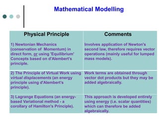
1) Newtonian Mechanics
(conservation of Momentum) in
direct form, or using 'Equilibrium'
Concepts based on d'Alembert’s
principle.
Comments
Involves application of Newton's
second law, therefore requires vector
operations (mainly useful for lumped
mass models).
2) The Principle of Virtual Work using
virtual displacements (an energy
principle using d'Alembert’s
principle).
Work terms are obtained through
vector dot products but they may be
added algebraically.
3) Lagrange Equations (an energy-
based Variational method - a
corollary of Hamilton's Principle).
This approach is developed entirely
using energy (i.e. scalar quantities)
which can therefore be added
algebraically.

2. Mathematical Modelling
THE LAGRANGE EQUATIONS.
What are they?
We have seen that it is possible to use a
different coordinate system to describe the
motion of a beam e.g.:
• A SDOF Lumped-mass model of a beam
(then using Newtonian Mechanics)
• A SDOF Generalised Displacement model of
beam structure motion obtained via the
Principle of Virtual Work.

3. THE LAGRANGE EQUATIONS.
i) Lumped mass
model
Z1(t) is the
generalised
coordinate
ii) Generalised
displacement
model
Z(t) is the
generalised
coordinate
The displacement of the system is only defined at the lumped mass by Z1;
The displacement is defined at all values of x , but Z(t) is still only a single variable.

4. THE LAGRANGE EQUATIONS.
We might ask: is it possible to write down the equations
of motion in terms of ‘generalised coordinates’ without
actually specifying what they are?
The answer is yes, i.e.: using Lagrange Equations.
The Lagrange Equations describe the dynamic behaviour
of systems with N-degrees-of-freedom in terms of energy
and (unspecified) ‘generalised coordinates’: q1,q1,…,qn.

5. THE LAGRANGE EQUATIONS.
In a particular application, say in modelling a
structure (whether lumped or distributed mass),
the particular coordinate system being used is
specified.
Note: if we take an N degree-of-freedom system
and obtain the equations of motion using different
coordinates, then although the resulting equations
will look different, the predicted (physical) motion
of the system will be identical.

6. THE LAGRANGE EQUATIONS.
Generalised coordinates
The term generalised coordinates can refer to any set of (coordinates), including
commonly used coordinates, which serve to specify the configuration of a system.
There is a relationship between the Number of Degrees of freedom and the
number of generalised coordinates i.e.:
The number of degrees-of-freedom (DOF) = The number of independent
coordinates needed to configure a system without violating any constraints.
or
The number of DOF = The number of Cartesian coordinates need to specify
system – the number of Cartesian equations of constraint.

7. THE LAGRANGE EQUATIONS.
Example: The Simple Pendulum (1-DOF system)
Ɵ is a generalised coordinate, whereas the Cartesian position (x,y) is subject to the constraint:
𝑥𝑥2 + 𝑦𝑦2 = 𝑟𝑟2

8. THE LAGRANGE EQUATIONS.
Lagrange Equations - detail
In defining the Lagrange equations an abstract set of independent generalised
coordinates is used: 𝑞𝑞1, 𝑞𝑞2, 𝑞𝑞3, … , 𝑞𝑞𝑛𝑛, where N is the number of degrees-of-
freedom. We can write down a set of N dynamical equations i.e. for each
coordinate 𝑞𝑞𝑖𝑖 in terms of the kinetic energy T and potential energy V:
𝑑𝑑
𝑑𝑑𝑑𝑑
𝜕𝜕𝜕𝜕
𝜕𝜕 ̇
𝑞𝑞𝑖𝑖
−
𝜕𝜕𝜕𝜕
𝜕𝜕𝑞𝑞𝑖𝑖
+
𝜕𝜕𝜕𝜕
𝜕𝜕𝑞𝑞𝑖𝑖
= 𝑄𝑄𝑖𝑖 𝑖𝑖 = 1,2, … , 𝑁𝑁
where the 𝑄𝑄𝑖𝑖 are known as the generalised forces representing non-
conservative or external forces (which cannot be represented in a particular
form i.e. cannot be derived from a potential function e.g. dissipative (damping
forces)). Absolute 𝑉𝑉 and 𝑇𝑇, or changes in V and T (Δ𝑉𝑉 and Δ𝑇𝑇) can be used.
If we have an N-degree-of-freedom system, we can write down N different
Lagrange equations, which apply to large (often nonlinear) displacements.

9. THE LAGRANGE EQUATIONS.
Special Cases
Conservative Systems:
This is the simplest case i.e.: when 𝑄𝑄𝑖𝑖 = 0 for all 𝑖𝑖.
Fixed Supports (Holonomic-scleronomic constraints):
For fixed constraints, the potential energy and kinetic
energy functions can usually be written: 𝑉𝑉 =
𝑉𝑉(𝑞𝑞1, 𝑞𝑞2, 𝑞𝑞3, … , 𝑞𝑞𝑛𝑛) and 𝑇𝑇 = 𝑇𝑇( ̇
𝑞𝑞1, ̇
𝑞𝑞2, ̇
𝑞𝑞3, … , ̇
𝑞𝑞𝑛𝑛) where
the generalised forces 𝑄𝑄𝑖𝑖 are defined such that a virtual
displacement of each generalised coordinate will produce
the correct total virtual work i.e. 𝛿𝛿𝛿𝛿 = ∑𝑖𝑖=1
𝑛𝑛
𝑄𝑄𝑖𝑖𝛿𝛿𝑞𝑞𝑖𝑖 (but
here treated as positive!).

10. THE LAGRANGE EQUATIONS.
Special Cases
If, in fact, we have force vectors 𝐹𝐹𝑖𝑖 defined in terms of
Cartesian Coordinates, which are related to the
generalised Coordinates as follows:
𝑥𝑥𝑗𝑗 = 𝜙𝜙𝑗𝑗(𝑞𝑞1, 𝑞𝑞2, … , 𝑞𝑞𝑁𝑁) 𝑗𝑗 = 1,2, … , 3𝑁𝑁
then it can be shown that:
𝑄𝑄𝑖𝑖 = �
𝑗𝑗=1
3𝑁𝑁
𝐹𝐹𝑗𝑗
𝜕𝜕𝑥𝑥𝑗𝑗
𝜕𝜕𝑞𝑞𝑖𝑖
(𝑖𝑖 = 1,2, … , 𝑁𝑁) (3𝐷𝐷)
where 𝐹𝐹𝑖𝑖 are the components of the force vectors
described in Cartesian Coordinates.

11. THE LAGRANGE EQUATIONS.
Example: Conservative 2DOF System
Here N= 2, the Generalised Coordinates are 𝑞𝑞1 ≡ 𝑥𝑥1 , 𝑞𝑞2 ≡ 𝑥𝑥2.
Kinetic energy 𝑇𝑇 =
1
2
𝑚𝑚1 ̇
𝑥𝑥1
2
+
1
2
𝑚𝑚2 ̇
𝑥𝑥2
2
and
Potential energy 𝑉𝑉 =
1
2
𝑘𝑘1𝑥𝑥1
2
+
1
2
𝑘𝑘(𝑥𝑥2 − 𝑥𝑥1)2
There are no external forces or dissipative forces ∴ 𝑄𝑄𝑖𝑖 = 0

12. THE LAGRANGE EQUATIONS.
The Lagrange equations are:
𝑑𝑑
𝑑𝑑𝑑𝑑
𝜕𝜕𝜕𝜕
𝜕𝜕 ̇
𝑥𝑥1
−
𝜕𝜕𝜕𝜕
𝜕𝜕𝑥𝑥1
+
𝜕𝜕𝜕𝜕
𝜕𝜕𝑥𝑥1
= 0
and
𝑑𝑑
𝑑𝑑𝑑𝑑
𝜕𝜕𝜕𝜕
𝜕𝜕 ̇
𝑥𝑥2
−
𝜕𝜕𝜕𝜕
𝜕𝜕𝑥𝑥2
+
𝜕𝜕𝜕𝜕
𝜕𝜕𝑥𝑥2
= 0
Assigning the specific terms in the Lagrange equations we have:
𝜕𝜕𝜕𝜕
𝜕𝜕 ̇
𝑥𝑥1
= 𝑚𝑚1 ̇
𝑥𝑥1;
𝑑𝑑
𝑑𝑑𝑑𝑑
𝜕𝜕𝜕𝜕
𝜕𝜕 ̇
𝑥𝑥1
= 𝑚𝑚1 ̈
𝑥𝑥1;
𝜕𝜕𝜕𝜕
𝜕𝜕 ̇
𝑥𝑥2
= 𝑚𝑚2 ̇
𝑥𝑥2;
𝑑𝑑
𝑑𝑑𝑑𝑑
𝜕𝜕𝜕𝜕
𝜕𝜕 ̇
𝑥𝑥2
= 𝑚𝑚2 ̈
𝑥𝑥2 and
𝜕𝜕𝜕𝜕
𝜕𝜕𝑥𝑥1
= 0;
𝜕𝜕𝜕𝜕
𝜕𝜕𝑥𝑥2
= 0;
𝜕𝜕𝜕𝜕
𝜕𝜕𝑥𝑥1
=
𝑘𝑘1𝑥𝑥1
−𝑘𝑘2(𝑥𝑥2 − 𝑥𝑥1)
;
𝜕𝜕𝜕𝜕
𝜕𝜕𝑥𝑥2
= 𝑘𝑘2(𝑥𝑥2 − 𝑥𝑥1)

13. THE LAGRANGE EQUATIONS.
Giving the usual equations of motion:
𝑚𝑚1 ̈
𝑥𝑥1 + 𝑘𝑘1𝑥𝑥1 − 𝑘𝑘2 𝑥𝑥2 − 𝑥𝑥1 = 0
and
𝑚𝑚2 ̈
𝑥𝑥2 + 𝑘𝑘2 𝑥𝑥2 − 𝑥𝑥1 = 0

14. THE LAGRANGE EQUATIONS.
EXTERNAL FORCES
How are the generalised forces 𝑄𝑄𝑖𝑖 established? If, in the
previous example, external forces 𝑓𝑓1(𝑡𝑡) and 𝑓𝑓2(𝑡𝑡) had been
applied to masses 𝑚𝑚1 and 𝑚𝑚2 then a virtual displacement 𝛿𝛿𝛿𝛿
would be made up of 𝛿𝛿𝑥𝑥1 and 𝛿𝛿𝑥𝑥2 so the total Virtual Work
done would be:
𝛿𝛿𝛿𝛿 = 𝑓𝑓1 𝑡𝑡 𝛿𝛿𝑥𝑥1 + 𝑓𝑓2(𝑡𝑡)𝛿𝛿𝑥𝑥2
since 𝑥𝑥1 = 𝑞𝑞1 𝑥𝑥2 = 𝑞𝑞2, this gives:
𝛿𝛿𝛿𝛿 = �
𝑖𝑖
𝑛𝑛
𝑄𝑄𝑖𝑖𝛿𝛿𝑞𝑞𝑖𝑖 = 𝑄𝑄1𝛿𝛿𝑞𝑞1 + 𝑄𝑄2𝛿𝛿𝑞𝑞2
We can identify the Generalised Forces 𝑄𝑄𝑖𝑖 (by association)
as 𝑄𝑄1= 𝑓𝑓1(𝑡𝑡) and 𝑄𝑄2 = 𝑓𝑓2(𝑡𝑡) appearing on the rhs of the
equations of motion.

15. THE LAGRANGE EQUATIONS.
Dissipative Forces (Damping)
These are non-conservative forces which can actually be absorbed
into the generalised forces 𝑄𝑄𝑖𝑖. It is possible to write down part of
the generalised forces in terms of a so called dissipation function:
𝐷𝐷 = 𝐷𝐷 ̇
𝑞𝑞1, ̇
𝑞𝑞2, … , ̇
𝑞𝑞𝑛𝑛
which contributes to the generalised force a term:
𝜕𝜕𝜕𝜕
𝜕𝜕 ̇
𝑞𝑞𝑖𝑖
Modified
Lagrange equations can then be written:
𝑑𝑑
𝑑𝑑𝑑𝑑
𝜕𝜕𝜕𝜕
𝜕𝜕 ̇
𝑞𝑞𝑖𝑖
−
𝜕𝜕𝜕𝜕
𝜕𝜕𝑞𝑞𝑖𝑖
+
𝜕𝜕𝜕𝜕
𝜕𝜕𝑞𝑞𝑖𝑖
+
𝜕𝜕𝜕𝜕
𝜕𝜕 ̇
𝑞𝑞𝑖𝑖
= 𝑄𝑄𝑖𝑖
Examples include the Rayleigh Dissipation function
𝐷𝐷 =
1
2
𝑐𝑐1 ̇
𝑞𝑞1
2
+ 𝑐𝑐2 ̇
𝑞𝑞2
2
+. .
which can be used to model linear viscous dampers (creating a
diagonal damping matrix).

16. THE LAGRANGE EQUATIONS.
Equations of Motion of a MDOF Linear Dynamic System
(undamped)
When considering a linear MDOF dynamic model for a
structure in terms of displacements, a linear system can be
shown to belong to a particular form when certain terms
are considered for the kinetic energy 𝑇𝑇 and potential
energy 𝑉𝑉. These forms can be established using either the
Lagrange equations or Virtual Work principles.

17. THE LAGRANGE EQUATIONS.
For small displacements (i.e. small amplitude oscillations) the
kinetic and potential energies can be expressed as so called
‘quadratic forms’ (i.e. for small movements about equilibrium
points, these terms follow from Maxwell’s Reciprocal Theorem
see Newland p314). The kinetic and potential energies are
written:
𝑇𝑇 =
1
2
∑𝑗𝑗=1
𝑁𝑁 ∑𝑖𝑖=1
𝑁𝑁
𝑚𝑚𝑖𝑖𝑖𝑖 ̇
𝑞𝑞𝑖𝑖 ̇
𝑞𝑞𝑗𝑗 =
1
2
̇
𝑞𝑞𝑇𝑇
𝑚𝑚 ̇
𝑞𝑞
And
𝑉𝑉 =
1
2
∑𝑗𝑗=1
𝑁𝑁 ∑𝑖𝑖=1
𝑁𝑁
𝜅𝜅𝑖𝑖𝑖𝑖𝑞𝑞𝑖𝑖𝑞𝑞𝑗𝑗 =
1
2
𝑞𝑞𝑇𝑇[𝜅𝜅]𝑞𝑞
where [𝑚𝑚] is the mass matrix, and [𝜅𝜅] is the stiffness matrix.

18. THE LAGRANGE EQUATIONS.
Now the usual Lagrange equations can be written in vector form
i.e.:
𝑑𝑑
𝑑𝑑𝑑𝑑
𝜕𝜕
𝜕𝜕 ̇
𝑞𝑞
𝑇𝑇 −
𝜕𝜕
𝜕𝜕𝑞𝑞
𝑇𝑇 +
𝜕𝜕
𝜕𝜕𝑞𝑞
𝑉𝑉 = 𝑄𝑄
where
𝜕𝜕
𝜕𝜕𝑞𝑞
=
𝜕𝜕
𝜕𝜕𝑞𝑞1
𝜕𝜕
𝜕𝜕𝑞𝑞2
𝜕𝜕
𝜕𝜕𝑞𝑞3
…
𝑇𝑇
and
𝜕𝜕
𝜕𝜕 ̇
𝑞𝑞
=
𝜕𝜕
𝜕𝜕 ̇
𝑞𝑞1
𝜕𝜕
𝜕𝜕 ̇
𝑞𝑞2
𝜕𝜕
𝜕𝜕 ̇
𝑞𝑞3
…
𝑇𝑇
are ‘operators’, and 𝑄𝑄 is a vector of generalised forces.

19. THE LAGRANGE EQUATIONS.
And since, as we have seen, the energy terms for a general linear
system in equilibrium, written in vector form, are:
�
𝑇𝑇 =
1
2
̇
𝑞𝑞𝑇𝑇 𝑚𝑚 ̇
𝑞𝑞
𝑉𝑉 =
1
2
𝑞𝑞𝑇𝑇[𝜅𝜅]𝑞𝑞
It can be shown that
𝜕𝜕𝜕𝜕
𝜕𝜕 ̇
𝑞𝑞𝑖𝑖
= [𝑚𝑚] ̇
𝑞𝑞 and therefore
𝑑𝑑
𝑑𝑑𝑑𝑑
𝑚𝑚 ̇
𝑞𝑞 = [𝑚𝑚] ̈
𝑞𝑞 and
that:
𝜕𝜕𝜕𝜕
𝜕𝜕𝑞𝑞𝑖𝑖
= [𝜅𝜅]𝑞𝑞. And since for a system with fixed constraints
𝜕𝜕𝜕𝜕
𝜕𝜕𝑞𝑞
= 0, then on substitution into the Lagrange Equations we get
the usual form of matrix differential equation:
𝒎𝒎 ̈
𝒒𝒒 + 𝒌𝒌 𝒒𝒒 = 𝑸𝑸
where all the non-conservative forces are absorbed into the
generalised force vector 𝑄𝑄 including all damping forces.

20. THE LAGRANGE EQUATIONS.
If damping forces can be modelled as linearly-dependent on
velocity e.g. using a Rayleigh dissipation function then a general
linear model, via Lagrange equations, takes the form:
𝑴𝑴 ̈
𝒒𝒒 + 𝑪𝑪 ̇
𝒒𝒒 + 𝑲𝑲 𝒒𝒒 = 𝑸𝑸(𝒕𝒕)
where 𝑄𝑄 now only includes external force components, which
are obtained individually by considering the work done 𝛿𝛿𝑊𝑊𝑖𝑖 by
(non-conservative) forces in going through some arbitrary Virtual
Displacements of each of the coordinates 𝛿𝛿𝑞𝑞1, 𝛿𝛿𝑞𝑞2, … , 𝛿𝛿𝑞𝑞𝑁𝑁.

21. Properties of the damping matrix [C]
Properties of the damping matrix [C]
Constructing the damping matrix of a complete structure is one of
the most difficult parts of the modelling process (even when
damping is linear).
However in choosing a (viscous) damping model which depends
linearly on the velocity, then the form of the chosen (Rayleigh)
model implies that the damping matrix is symmetric i.e. 𝑐𝑐𝑖𝑖𝑖𝑖 = 𝑐𝑐𝑗𝑗𝑗𝑗 or
[𝐶𝐶]𝑇𝑇= [𝐶𝐶].
But in practice, for real structures, damping matrices are rarely
obtained other than by some sort of experimental calibration
process which is often based on specific assumptions.

22. A very important assumption which allows the equations of
motion to be solved using so called Normal Coordinates, is to
assume damping is proportional to either the stiffness matrix
[K] or the mass matrix [M], or in general, both i.e. assume:
𝐶𝐶 = ∝ 𝑀𝑀 + 𝛽𝛽[𝐾𝐾]
where ∝ and 𝛽𝛽 are constant (scalars). This type of damping
model is known as ‘proportional damping’. We will return to
the use of this important damping model soon.
Proportional Damping