The greedy method constructs an optimal solution in stages by making locally optimal choices at each stage without reconsidering past decisions. It selects the choice that appears best at the current time without regard for its long-term consequences. The general greedy algorithm procedure selects the best choice from available inputs at each stage until a complete solution is reached. Examples demonstrate both when the greedy method succeeds in finding an optimal solution and when it fails to do so compared to alternative methods like dynamic programming.
1. The greedy method
In the greedy method we attempt to construct an optimal solution in stages. At each
stage we make a decision that appears to be the best at that time ( optimal one ). A
decision made in one stage is not changed later and should assure feasibility ( i.e it must
satisfy all constraints ). It is called ‘greedy’ because it chooses the best one at that stage
without considering whether this will prove to be a sound decision in the long run.
General Method
Procedure GREEDY(A,n)
Solutionnull
for I 1 to n do
x SELECT(A)
if FEASIBLE(Solution,x)
then Solution UNION(Solution,x)
end if
repeat
return(Solution)
end GREEDY
A is a set of all possible inputs
SELECT function selects a input from A
FEASIBLE determines whether x can be included into the solution vector
UNION combines x with solution and updates the objective function
Example:
Suppose we are living in a place having coins of 1, 4, and 6 units we want to
make change of 8 units, we greedily select one 6 units and 2 one units instead of
selecting two 4 units which is a better solution.
Example:
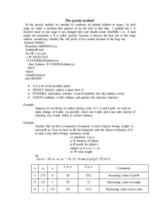
Assume that we have a knapsack of capacity m and n objects having weight wi
and profit pi. Now we have to fill the knapsack with the object or fraction of it
in such a way that it brings maximum profit.
i.e maximize pi xi
xi fraction of object
pi profit for object i
subject to xi wi < = m
m total weight
eg:
Let m = 20, w1, w2, w3 = 18, 15, 10 and p1,p2,p3 =25,24,15
xi xi xi
wi xi pi xi
Comments
1 2/15 0 20 28.2 Increasing order of profit
0 2/3 1 20 31 Decreasing order of weight
0 1 1/2 20 31.5 Decreasing order of p/w ratio
2. From the above example we see that we can get the maximum profit by
arranging the elements in the decreasing order of p/w ratio.
Procedure GREEDY_KNAPSACK
(Assume the objects are arranged in the decreasing order of p/w ratio)
x 0
remweight m
for i 1 to n do
if w(i) > remweight then exit
end if
x(i) 1
remweight remweight – w(i)
repeat
if i < = n then x(i) remweight/w(i)
end if
end GREEDY_KNAPSACK
Efficiency in terms of time without considering time to sort is O(n)
x is an array representing solutions
remweight denotes remaining weight initialized to m first
Example 2:
Minimum spanning tree:
Given an n – vertex undirected network G having n-1 edges, our problem is to
select n-1 edges in such a way that selected edges form a least cost spanning
tree.
There are two different greedy techniques to solve this problem:
(1) Kruskals
(2) Prims
Kruskals Algorithmn:
General method:
From the remaining edges we select a least cost edge that does not result in a
cycle when added to the set of already selected edges.
Consider:
4
3
2
1
6
7
5
24
0
28
28
0
25
0
22
0
12
0
16
0
14
0
10
18
0
3. First arrange the edges in the ascending order of cost.
{1,6},{3,4},{2,6},{2,3},{7,4},{5,4},{5,7},{6,5},{1,2}
We will now strart constructing the shortest path according to Kruskal’s
algorithmn.
1. Add {1,6}
2. Add {3,4}
3. Add {2,7}
4
3
2
1
6
7
5
10
4
3
2
1
6
7
5 12
0
10
4
3
2
1
6
7
5 12
0
14
0
10
5. Function Kruskal
Sort all the edges by increasing order of weights
N number of weights
T null
Repeat
e {u,v} // Shortest edge not yet considered
ucomp find(u) //find(u) tells us to which component does u belong to
vcomp find(v)
if ucomp <> vcomp then //doesn’t form a cycle
merge(ucomp,vcomp)
T T U {e}
Until T contains n-1 edges
Return T
Time taken for this algorithm is O(alogn)
A number of edges
N number of nodes
Example:
From the remaining edges select a least cost edge whose addition to the set of
selected edges forms a tree.
Consider the following example as that of kruskals:
4
3
2
1
6
7
5
10
4
3
2
1
6
7
5
25
0
10
4
3
2
1
6
7
5
25
0
22
0
10
4
3
2
1
6
7
5
25
0
22
0
12
0
10
6. Efficiency of the algorithm is O(n2)
Algorithm PRIMS(E,COST,n,T,mincost)
(k,l) edge with minimum cost;
mincost COST(k,l)
T[1,1] k;
T[1,2] l;
For i 1 to n do
If COST(i,l) < COST(I,k) then
NEAR(i) l
Else
NEAR(i) k
End if
Repeat
NEAR(l) NEAR(l) 0
For i 2 to n-1 do
If NEAR(j) 0 and COST(j,NEAR(j)) is minimum
T[i,1] j;
T[I,2] NEAR(j);
mincost mincost + COST(j,NEAR(j))
NEAR(j) 0
For k1 to n do
If NEAR(k) 0 and COST(k,NEAR(k)) > COST(k,j)
Then NEAR(k) j
End if
Repeat
Repeat
If mincost then print (‘no spanning tree’) end if
End PRIM
4
3
2
1
6
7
5
25
0
22
0
12
0
16
0
10
4
3
2
1
6
7
5
25
0
22
0
12
0
16
0
14
0
10
7. Dynamic Programming method
It is a bottom up approach in which we avoid calculating the same thing twice by keeping
a table of known results that fills up as sub instances are solved. In greedy method we
make irrevocable decisions one at a time using greedy criteria but there here we examine
the decision sequence to see whether the optimal decision sequence contains optimal
decision subsequences. These optimal sequences of decisions are arrived by making use
of the PRINCIPLE OF OPTIMALITY.
This principle states that an optimal sequence of decisions has the property that whatever
the initial state and decisions are the remaining decisions must constitute an optimal
decision sequence with regard to the state resulting from the first decision.
Example:
Making changes:
Suppose we live in an area where there are coins for 1, 4, 6 units . If we have to
make change for 8 units the greedy algorithm will propose one 6 unit and two 1
unit coins making a total of three coins. The better solution is giving two 4 unit
coins.
To solve this problem by dynamic programming we assume a table [1..n,0..N]
One row for each denomination [1---n]
One column for each amount [1---N]
C[i,j] will be the minimum number of coins required to pay an amount
of j units using only denominations from 1 to i.
To pay an amount j using coins of denominations 1 to I we have 2
choices
1. First we may choose not to use any coins of that denominations i
that is C [i , j]=C[i-1,j]
2. we may choose to use atleast one coin of this denomination
hence
C[i,j]=one coin from this denomination+least number of
coins that make up the rest of the amount i.e j-di
= 1 + C[i,j-di]
In general C[i,j] = min( C[i-1,j],1+C[i,j-di])
i – denomination row
j – amount requiring change
8. AMOUNT/
DENOMINATION 0 1 2 3 4 5 6 7 8
d1=1 0 1 2 3 4 5 6 7 8
d2=4 0 1 2 3 1 2 3 4 2
d3=6 0 1 2 3 1 2 1 2 2
The above table is the cost matrix C[3,9]
C[i,j] – The number of coins needed to make change for j unit using
denominations less than or equal to dj.
From this table if we want to find out the number of minimum coins to make an
amount of 7 units with only 2 denominations then we look up at C[2,7] we get 4
coins one 4 unit coins and 3 one unit coins
C[1,0]=0
C[1,1]=C[1,0]+1=1 since C[0,0] is not possible we cannot consider min(C[0,0],1+C[1,0])
C[2,0]=C[1,0] = 0
C[2,6]=min(C[2,6-4]+1,C[1,6])=min(C[2,2]+1,C[1,6])=min(2+1,6)=3
C[3,8]=min(C[3,8-6]+1,C[2,8])=min(C[3,2]+1,C[2,8])=min(2+1,2)=2
Algorithm:
Function Coins(N)
(gives minimum number of coins to make change for N units)
for i 1 to n do C[i,0] 0 //for the amount 0 the change required
for i 1 to n do
for j 1 to N do
C [I,j] (if i =1 and j<d[i] then +
Else if i=1 then 1+C [1,j-d [1]]
Else if j<d [i] then C [i-1,j]
Else min(C [i-1,j],1+C[i,j-d[i]])
Return C[n,N]
The total time required for this algorithm is O(n, C[n,N])
n Number of denominations
N amount
Example:
0/1 Knapsack problem:
Assume that we have a knapsack of capacity m and n objects having weight wi
and profit pi. Now we have to fill the knapsack with the object or we discard it,
(We allow no fractions)t in such a way, that it brings maximum profit.
i.e maximize pi xi
xi 0 or 1
pi profit for object i
subject to xi wi < = m
m total weight
Similar to the previous problem we create a table V[1…n,0…w] with one row
for each available object and one column for each weight from 0 to w
9. The criterion for filling the table depends upon two choices
1. adding the object .
2. Neglecting the object.
Let us assume that we have five objects of weights 1, 2, 5, 6, and 7 units
having a profit of 1, 6, 18, 22, and 28 respectively. We have to fill a knapsack
in such a manner the total weight of the objects does not exceed the maximum
capacity of the knapsack i.e. 11 units.
CAPACITY
/WEIGHT 0 1 2 3 4 5 6 7 8 9 10 11
w1=1,p1=1 0 1 1 1 1 1 1 1 1 1 1 1
w2=2,p2=6 0 1 6 7 7 7 7 7 7 7 7 7
w3=5,p3=18 0 1 6 7 7 18 19 24 25 25 25 25
w4=6,p4=22 0 1 6 7 7 18 22 24 28 29 29 40
w5=7,p5=28 0 1 6 7 7 18 22 28 29 34 35 40
In the above table construction we have assumed the following formula
v[i, j] = max ( v[i-1, j], v[i-1, j-wi] + pi )
each v[i, j] = pi of selected objects
v[4, 7] = max ( v[3,7], v[3, 7-6]+22)=max ( 24,1+22)=24
In the above example it was more profitable to put one object of w3=5 and
one object of w2=2 to get a profit of p2+p3=18+6, rather than just putting in
one object of w4=6 and one object of w1 = 1 to get a profit of p4+p1=22+1.
Example:
Traveling salesman problem:
This problem deals with finding a tour of minimum cost covering all the nodes in
a weighted undirected graph, starting and ending at a particular node.
Similar to the previous examples, here also we make use of one function to deal
with the principle of optimality i.e.
g(i,S) = min { Cij+ g(j, S – {j})}
g( I, s) minimum cost of traveling from node i and covering all the nodes in
S and reaching back to the node i.
Cij denotes cost of going from node i to node j
S the set of all nodes except node i
S – {j} set of all nodes except nodes i and j
Suppose we want to find a minimum path from node 1 covering all the nodes
in set V and coming back to node 1, we denote it by
g(1,V-{1}) = min(cik+g(k,V-{1,k})} 2 k n
n number of nodes
10. Consider the cost Matrix of the salesman
Now let us try to find the minimum path starting at node 1 and ending at the same
node and covering all the other nodes.
g(1,{2, ,3, 4}) = min {C12+ g(2,{3, 4}),C13+g(3,{2,4}),C14+g(4,{2,3})}
= min (10+25,15+25,20+23)
= 35
g(2,{3, 4}) = min {C23+ g(3,{4}),C24+g(4,{3})}=min(9+20,10+15) =25
g(3,{2, 4}) = min {C32+ g(2,{4}),C34+g(4,{2})}=min(13+18,12+13)=25
g(4,{2, 3}) = min {C42+ g(2,{3}),C43+g(3,{2})}=min(8+15,9+18) =23
g(3,{4}) = C34+g{4,}=12+8 =20
g(4,{3}) = C43+g{3,}=9+6 =15
g(2,{4}) = C24+g{4,}=10+8 =18
g(4,{2}) = C42+g{2,}=8+5 =13
g(2,{3}) = C23+g{3,}=9+6 =15
g(3,{2}) = C32+g{2,}=13+5 =18
g{2,}=C21=5; g{3,}=C31=6; g{4,}=C41=8;
The required cost is g(1,{2,3,4}) = 35
Path is 1 2 4 3 1
Efficiency is in terms of time is O(n22n)
0 10 15 20
5 0 9 10
6 13 0 12
8 8 9 0
1
2
3
4
1 2 3 4
11. Backtracking
This method is based on the systematic examination of the possible solutions. We have
a procedure that looks thorough the set of possible solutions and the possible solutions
are rejected even before they are completely examined hence the number of possible
solutions are getting smaller. We reject solutions on the basis that certain solutions do not
fulfill certain requirements set beforehand. The name backtracking was coined by
Dr.Lehmer.
We have a finite set of solution space Si each element in the solution space is given as a
n - tuple (x1,x2,….,xn) and a certain set of constraints to be satisfied by any of the
solutions in the solution space.
Constraints are categorized into implicit and explicit constraints. Explicit constraints
are rules that restrict each xi to take on values from a given set. Eg: each xi > 0
Implicit constraints are rules that determine which tuple satisfy the criterion function.
Example:
N Queens problem:
N queens are to be placed on a n x n chessboard so that no two attack. Generally
we have n! Permutation possibilities.
Let us consider for n=4 we have 24 possibilities. We will construct a tree
structure to represent all the possibilities. In the following tree the 1st level is for
the first row in the chessboard and the 2nd level for the 2nd row and so on.
12. Q
Q
Q
Dead end Hence Backtrack Dead end hence Backtrack
Q
Q
Q
Q
Solution
Algorithm Nqueens(k,n)
{it gives all possible placements of n queens on an n x n Matrix)
{
for(I=1 to n do
{
if Place(k,I) then
{
x[k] := I
if(k==n) then Write(x[i:n])//Solution found all queens placed
else Nqueens(k+1,n)
}
}
}
Algorithm Place(k,I)
{returns true if a queen can be placed in k th row and i th column)
{
for j=1 to k-1 do
if (x[j] = I or (Abs(x[j] –1) = Abs(j-k)) then
return false
else return true;
}
Q
Q
13. The algorithm Nqueens can be invoked by calling NQueens(1,n)
To place a queen on the chessboard we have to check for three conditions
1. Must not be on the same row
2. Must not be in the same column
3. Must not remain in the same diagonal
Suppose 2 queens are placed at the positions (i,j) and (k,l) then
i-j=k-l
These computations are verified in the algorithm.
The computing time of the algorithm Place is O(k-1).
Example
Graph coloring:
Let G be a graph and m be a given positive integer.We have to color the nosdes of G in
such a way so that no two adjacent nodes have the same color, yet only m colors are
being used. Chromatic number indicates smallest integer m for which the graph can be
colored. Here we use backtracking technique to color a given graph using atmost m
colors.
Assume that our graph is represented by an adjacency matrix GRAPH(1…n,1..n) where
GRAPH(i,j)= true or 1 if thee exists an edge between node i and node j otherwise it is 0
or false. The colors are represented by integers 1….m .Solution is given by an array x[]
where x[I] gives the color of the node i.
Consider:
1 2
4
3
5
1
2
1
3
3
0 1 1 0 1
1 0 1 0 1
1 1 0 1 0
0 0 1 0 1
1 1 0 1 0
1
2
3
4
5
1 2 3 4 5
14. The Graph in the figure can be colored by 3 colos as indicated ihn the figue.
Solution is:
x[1]=1, x[2]=2, x[3]=3, x[4]=1, x[5]=3
Algorithm mcoloing(k)
(k ios the index of the next vector to be colored)
{
}