SlideShare une entreprise Scribd logo
1  sur  724
Télécharger pour lire hors ligne
Chapter 1 - Section A - Mathcad Solutions
1.4 The equation that relates deg F to deg C is: t(F) = 1.8 t(C) + 32. Solve this
equation by setting t(F) = t(C).
Guess solution:

t

t = 1.8t

Given

0

Find t
()

32

Ans.

40

P=

1.5 By definition:

F
A

F = mass g

A

P

3000bar

D

4mm

F

PA

g

9.807

m

D

4

F

mass

2

g

s

P=

1.6 By definition:

F
A

A

3000atm

D

0.17in

F

PA

g

32.174

ft

4

D

mass

2

sec

gh

13.535

1.8

gm
3

101.78kPa

13.535

g

9.832

mass

2

384.4 kg

Ans.

2

F
g

A

mass

2

0.023 in

1000.7 lbm

Ans.

gm
3

29.86in_Hg

m

h

2

56.38cm

s

Pabs

g

gh

32.243

Patm

ft

Pabs

h

2

176.808 kPa Ans.

25.62in

s

cm

Patm

12.566 mm

Patm

cm

Patm

A

F = mass g

P

1.7 Pabs =

2

Note: Pressures are in
gauge pressure.

Pabs

gh

1

Patm

Pabs

27.22 psia

Ans.
1.10 Assume the following:

13.5

gm

g

3

m

9.8

2

s

cm

P

1.11

P

h

400bar

h

g

Ans.

302.3 m

The force on a spring is described by: F = Ks x where Ks is the spring
constant. First calculate K based on the earth measurement then gMars
based on spring measurement on Mars.
On Earth:

F = mass g = K x

mass

g

0.40kg

9.81

m

x

2

1.08cm

s

F

F

mass g

F
x

Ks

3.924 N

Ks

363.333

N
m

On Mars:

x

0.40cm

gMars

1.12 Given:

FMars

gMars

FMars
mass

d
P=
dz

g

0.01

FMars

Kx

and:

mK

=

4

MP
RT

Substituting:

Separating variables and integrating:

1
dP =
P

Psea

1atm

ln

M

29

2

mK

PDenver
Psea

=

PDenver = Psea e
gm
mol

d
P=
dz

zDenver

Mg
zDenver
RT
Mg
zDenver
RT

g

9.8

MP
g
RT

Mg
dz
RT

0

Psea

Taking the exponential of both sides
and rearranging:

3

Ans.

kg

PDenver

After integrating:

10

m
2

s
3

R

82.06

cm atm

T

mol K

Mg
zDenver
RT
Mg
RT

(
10

zDenver

273.15)
K

0.194

zDenver

Psea e

PDenver

0.823 atm

Ans.

PDenver

PDenver

1 mi

0.834 bar

Ans.

1.13 The same proportionality applies as in Pb. 1.11.

gearth

ft

32.186

gmoon

2

5.32

M

lmoon

1.14

gearth
gmoon

costbulb

Ans.

18.767 lbf

Ans.

hr
0.1dollars
70W
10
day
kW hr

hr
5.00dollars
10
day
1000hr

costelec

dollars
yr

costelec

25.567

dollars
yr

costtotal

43.829

dollars
yr Ans.

18.262

costtotal

costbulb

D

18.76

113.498

113.498 lbm

wmoon

M gmoon

costbulb

1.15

learth

M

learth lbm

wmoon

lmoon

2

s

s

learth

ft

1.25ft

costelec

mass

250lbm

g

32.169

ft
2

s

3
Patm

(a) F

30.12in_Hg

Patm A

l

Work

1.7ft

D

D

2

3

10 lbf

Work

PE

mass g l

mass

1.227 ft

2

Ans.

Ans.

16.208 psia

F l

0.47m

A

2.8642

Pabs

PE

1.16

4

F

mass g

F
A

(b) Pabs

(c)

A

3
10 ft lbf Ans.

4.8691

Ans.

424.9 ft lbf

g

150kg

9.813

m
2

s

Patm

(a) F

Patm A

l

0.83m

EP

1.18

mass

EK

2

A
4

110.054 kPa

Work

EP

mass g l

u

1250kg

1
2
mass u
2

40

EK

m
s

Work

EK

Wdot =

200W

Ans.

1000 kJ

mass g h
0.91 0.92
time

Wdot

Ans.

1000 kJ

g

9.8

m
2

s

4

h

2

0.173 m

Ans.

10 N

F l

Work

1.19

1.909

Pabs

Work

D

4

F

mass g

F
A

(b) Pabs

(c)

A

101.57kPa

50m

Ans.

15.848 kJ Ans.

1.222 kJ

Ans.
Wdot

mdot

1.22
a) cost_coal

mdot

g h 0.91 0.92

0.488

25.00
ton

cost_coal

MJ
29
kg

cost_gasoline

0.95 GJ

kg
s

1

2.00
gal

37

GJ

cost_gasoline

Ans.

14.28 GJ

1

3

m

cost_electricity

0.1000
kW hr

cost_electricity

27.778 GJ

1

b) The electrical energy can directly be converted to other forms of energy
whereas the coal and gasoline would typically need to be converted to heat
and then into some other form of energy before being useful.
The obvious advantage of coal is that it is cheap if it is used as a heat
source. Otherwise it is messy to handle and bulky for tranport and
storage.
Gasoline is an important transportation fuel. It is more convenient to
transport and store than coal. It can be used to generate electricity by
burning it but the efficiency is limited. However, fuel cells are currently
being developed which will allow for the conversion of gasoline to electricity
by chemical means, a more efficient process.
Electricity has the most uses though it is expensive. It is easy to transport
but expensive to store. As a transportation fuel it is clean but batteries to
store it on-board have limited capacity and are heavy.

5
1.24 Use the Matcad genfit function to fit the data to Antoine's equation.
The genfit function requires the first derivatives of the function with
respect to the parameters being fitted.
B
T C

A

Function being fit:

f ( A B C)
T

e

First derivative of the function with respect to parameter A

d
f ( A B C)
T
dA

B

exp A

T

C

First derivative of the function with respect to parameter B

d
f ( A B C)
T
dB

1
T

C

B

exp A

T

C

First derivative of the function with respect to parameter C

d
f ( A B C)
T
dC

B
(
T

2

exp A

C)

18.5

3.18

9.5

5.48

0.2
11.8
t

9.45
16.9

23.1
32.7

Psat

28.2
41.9

44.4

66.6

52.1

89.5

63.3

129

75.5

187

6

B
T

C
T

t

273.15

lnPsat

ln ( )
Psat

Array of functions used by Mathcad. In this case, a0 = A, a1 = B and a2 = C.

exp a0
exp a0

F ( a)
T

a1
T

a2
a1

T

1
exp a0
T a2
a1
T

a2

2

Guess values of parameters

15

a2

guess

a1
T

exp a0

3000
50

a2
a1
T

a2

Apply the genfit function

A

13.421

A

B

B

genfit ( Psat guess F)
T

C

2.29

C

3

10

Ans.

69.053

Compare fit with data.
200

150
Psat
f ( A B C)
T

100

50

0
240

260

280

300

320

340

360

T

To find the normal boiling point, find the value of T for which Psat = 1 atm.

7
Psat

1atm

B

Tnb
A

Tnb
1.25
a) t1

1970

C2

C1 ( 1

t2
i)

273.15K

2000

dollars
gal

C1

0.35

1.513

329.154 K

Ans.

56.004 degC

C2

t2 t1

Tnb

C K

Psat
ln
kPa

i

5%

dollars
gal

The increase in price of gasoline over this period kept pace with the rate of
inflation.
b) t1

1970
Given

t2
C2
C1

= (1

2000
i)

C1

t2 t1

i

16000

dollars
yr

Find ( i)

i

C2

80000

dollars
yr

5.511 %

The salary of a Ph. D. engineer over this period increased at a rate of 5.5%,
slightly higher than the rate of inflation.
c) This is an open-ended problem. The strategy depends on age of the child,
and on such unpredictable items as possible financial aid, monies earned
by the child, and length of time spent in earning a degree.

8
Chapter 2 - Section A - Mathcad Solutions
2.1 (a)

Mwt

g

35 kg

9.8

m

z

2

5m

s

Work

(b)

Work

Mwt g z

Utotal

Utotal

Work

(c) By Eqs. (2.14) and (2.21):

dU

1.715 kJ Ans.

1.715 kJ

Ans.

d ( )= CP dT
PV

Since P is constant, this can be written:

MH2O CP dT = MH2O dU

MH2O P dV

Take Cp and V constant and integrate: MH2O CP t2 t1 = Utotal
kJ
MH2O 30 kg
CP
4.18
t1 20 degC
kg degC
t2

t1

Utotal
MH2O CP

t2

20.014 degC Ans.

(d) For the restoration process, the change in internal energy is equal but of
opposite sign to that of the initial process. Thus

Q

(e)

Utotal

Q

1.715 kJ

Ans.

In all cases the total internal energy change of the universe is zero.

2.2 Similar to Pb. 2.1 with mass of water = 30 kg.
Answers are:

(a) W = 1.715 kJ
(b) Internal energy change of
the water = 1.429 kJ
(c) Final temp. = 20.014 deg C
(d) Q = -1.715 kJ
9
2.4

The electric power supplied to the motor must equal the work done by the
motor plus the heat generated by the motor.

E

i 9.7amp

Wdotelect

Qdot

2.5

i
E

Wdotelect
t

Eq. (2.3):

U = Q

Step 1 to 2:

Ut12

Wdotelect

1.067

3

134.875 W

Ans.

W

W12

200J

Ut12

Q34

Q12

800J

Ut34

1.25hp

10 W

Qdot

Wdotmech

Q12

Step 3 to 4:

Wdotmech

110V

W12

6000J

W34

Q34

Ut34

W34

3

5.8

Ans.

10 J

300J

Ans.

500 J
t

t

Step 1 to 2 to 3 to 4 to 1: Since U is a state function, U for a series of steps
that leads back to the initial state must be zero. Therefore, the sum of the
t

U values for all of the steps must sum to zero.

Ut41

4700J

Ut23
Step 2 to 3:

Ut23

W23

Ut34

Ut41

Ans.

4000 J

Ut23

Ut12

4

Ut23

3

Q23

Q23

3800J

W23

10 J

200 J

Ans.

For a series of steps, the total work done is the sum of the work done for each
step.

W12341

1400J
10
W41

W12341

Step 4 to 1:

W12

W23

Ut41

Ut41

Ans.

10 J
3

4.5

Q41

W41

3

4.5

W41

4700J

Q41

Note:

W41

W34

10 J

200 J

Ans.

Q12341 = W12341

2.11 The enthalpy change of the water = work done.

M

Wdot

2.12 Q

CP

20 kg

4.18

kJ
kg degC

t

10 degC

M CP t

0.25 kW

0.929 hr

Wdot

Ans.

U

Q

12 kJ

W

U

19.5 kJ

Ans.

Q

12 kJ

U

W

U

7.5 kJ

Q

12 kJ

Ans.

2.13Subscripts: c, casting; w, water; t, tank. Then

mc Uc

mw Uw

mt Ut = 0

Let C represent specific heat,

C = CP = CV

Then by Eq. (2.18)

mc Cc tc

mw Cw tw

mt Ct tt = 0

mc

2 kg

mw

Cc

0.50

kJ
kg degC

Ct

mt

40 kg

tc

500 degC

Given

t1

mc Cc t2

t2

0.5

5 kg

kJ
kg degC

Cw

25 degC

t2

30 degC

tc = mw Cw

mt Ct

t2

Find t2
11

t2

4.18

kJ
kg degC

(guess)

t1

27.78 degC

Ans.
2.15

mass

(a)

(b)

T

g

CV

1 kg

Ut

1K

9.8

m

Ut

mass CV T

EP

2

kJ
kg K

4.18

Ans.

4.18 kJ

Ut

s

z

(c)

2.17

EP

EK

z

z

mass g

426.531 m Ans.

EK

u

Ut

1
mass
2

1000

50m

u

kg

5

A

3

A

2m

mdot

Wdot

uA

mdot

mdot g z Wdot

4

D

2

(b)

2

4 kg

1.571 10

7.697

s
3

10 kW

U1

P1

1002.7 kPa

U1

H1

763.131

U2

kJ
2784.4
kg

H2

U2

P1 V 1

kJ
kg

kJ
kg

cm
1.128
gm

V1

Ans.
3

P2

U

P2 V 2

2022.4

Ans.
3

kJ
762.0
kg

U

Ans.

3.142 m

H1

2.18 (a)

m
s

m
s

u

m

D

91.433

Ans.

1500 kPa

U2

U1

H

12

cm
169.7
gm

V2

H

2275.8

kJ
kg

H2

H1

Ans.
2.22

D1

(a)

u1

2.5cm

m
s

D2

5cm

For an incompressible fluid, =constant. By a mass balance,
mdot = constant = u 1A1 = u2A2

u2
(b)

D1

u1

u2

D2
1

EK

2

2

2

u2

1
2

2.23 Energy balance:

Mass balance:

u1

2

mdot3 H3

mdot1

1.0

Qdot

30

Qdot

H1

T1

CP

4.18

s

mdot1

mdot2 H2 = Qdot

H2 = Qdot

mdot2 CP T3

25degC

kJ

Ans.

kg

mdot2 H3

T1

kg
s

J

mdot2 = 0

mdot2 = Qdot

mdot1 CP T1

Ans.

1.875

mdot1

mdot Cp T3

T3 CP mdot1

m
s

mdot1 H1

mdot1 H3

or

0.5

EK

mdot3

Therefore:

T3

2

T2 = Qdot

mdot1 CP T1

mdot2 CP T2

mdot2

0.8

kg
s

T2

75degC

kJ
kg K

mdot2 CP T2

mdot2 CP

T3

43.235 degC

2

2.25By Eq. (2.32a):

By continuity,
incompressibility

H

u
= 0
2
A1

u2 = u1

13

A2

H = CP T

CP

4.18

kJ
kg degC

Ans.
2
u = u1

u1

u1

2

2 CP

D2

2
u = u1

1

m
s

14

D1

D1

2

1

A2

SI units:

T

2

A1

2

4

1

D2

D1

D2

2.5 cm

3.8 cm

4

T

0.019 degC

Ans.

T

D2

0.023 degC

Ans.

7.5cm

u1

T

2

2 CP

D1

1

4

D2

Maximum T change occurrs for infinite D2:

D2

cm

u1

T

2.26 T1

2 CP

300K

Wsdot

H

2

D1

1

T

D2

T2

u1

520K

ndot

98.8kW

CP T2

4

50

H

T1

10

0.023 degC

m
s

u2

kmol
hr

3.5

10

molwt

29

kg
kmol

7
R
2

CP

6.402

m
s

Ans.

3 kJ

kmol

By Eq. (2.30):

Qdot

H

2

u2
2

2

u1
2

molwt ndot

Wsdot Qdot

2

2.27By Eq. (2.32b):

By continunity,
constant area

H=

u2 = u1

u

2 gc

V2

u2 = u1

V1
14

also

T 2 P1
T 1 P2

Ans.

9.904 kW

V2
V1

=
2

T 2 P1
T 1 P2
2

u = u2

u1

2
2
u = u1

P1

R

T2

T2

P2

molwt

mol rankine

7
2

u1

20 psi

ft lbf

28

20

7
R T2
2

ft
s

T1

T1

579.67 rankine

H2

2726.5

kJ
kg

kJ
kg

Ans.

gm
mol

(guess)

578 rankine

Given

H = CP T =

1

T 1 P2

100 psi

3.407

2

T 2 P1

2

2

R T2

T1 =
T2

Find T2

u1
2

2

T 2 P1
T 1 P2

1 molwt

Ans.

578.9 rankine

(
119.15 degF)

2.28 u1

3

m
s

u2

200

m
s

H1
2

By Eq. (2.32a):

2.29 u1

u2

m
s
m
500
s

30

By Eq. (2.32a):

Q

H2

H1

3112.5

u1

u2

H1

334.9

kJ
kg

2

Q

2

kJ

H2

kg

2411.6

2945.7

(guess)
2

H2

Given

u2

578.36

m
s

H1 =

u2

u1

2

5 cm

V1

388.61

u2

2

Ans.
3

3

D1

kJ
kg

cm

gm
15

V2

667.75

cm

gm

Find u2
Continuity:

2.30 (a)

t1

D2

t2

30 degC

CV

u1 V2
u2 V1

D1

D2

Ans.

1.493 cm

n

250 degC

3 mol

J
mol degC

20.8

By Eq. (2.19):

Q

n CV t2

Q

t1

Ans.

13.728 kJ

Take into account the heat capacity of the vessel; then

cv

mv

Q

(b)

100 kg

mv cv

t1

200 degC

CP

29.1

n CV

CV

Q

Q

Ans.

11014 kJ

n

40 degC

4 mol

joule
mol degC
Q

n CP t2

t2

70 degF

5

kJ
kg degC

t1

t2

By Eq. (2.23):

2.31 (a) t1

t2

0.5

BTU
mol degF

n CV t2

Q

t1

18.62 kJ

n

350 degF

3 mol

By Eq. (2.19):

Q

t1

4200 BTU

Ans.

Take account of the heat capacity of the vessel:

mv

Q

mv cv

cv

200 lbm

(b) t1

400 degF

n CV

t2

0.12

BTU
lbm degF

Q

t1

t2

150 degF

16

10920 BTU

n

Ans.

4 mol

Ans.
CP

7

BTU
mol degF

Q

H1

2.33

n CP t2

1322.6

V1

Q

t1

BTU

BTU
lbm

1148.6

3

V2

lbm

78.14

ft

4

mdot

mdot

V2

10

22.997

u2

Wdot

2.34

H1

V1

H2

307

9.25

BTU
lbm

ft

H2

330

V2

u1

lbm

ft

0.28

173.99

BTU
lb

Ans.

39.52 hp

BTU

3

lbm

Ws

2

Wdot

Ws mdot

u1

u2

H1

20

ft
s

molwt

44

3

D1

lbm

D2

4 in

1 in

2

mdot

u2

4

D1 u1

mdot

V1

V2

mdot

u2

679.263

9.686

2

4

D2

2

Eq. (2.32a): Q

H2

H1

10 in

sec

2

D2

Eq. (2.32a): Ws

D2

ft
sec

2

4

3 in

4 lb

3.463

V1

mdot

10

D1

lbm

2

u2

ft
s

u1

3

2

D 1 u1

Ans.

7000 BTU

H2

lbm

ft

3.058

By Eq. (2.23):

ft
sec

u1

u2

2
17

lb
hr

2

Ws

Ws
molwt

5360

Q

BTU
lbmol

98.82

BTU
lbm

gm
mol
Qdot

2.36

T1

Qdot

mdot Q

P

300 K

67128

BTU
hr

Ans.

1 kg

n

1 bar

28.9

V1

n

gm

34.602 mol

mol
3

3
bar cm T1
83.14
mol K P

cm
24942
mol

V1

V2

P dV = n P V 1

W= n

V2 = n P V1

3 V1

V1

Whence

W

Given:

V2
V1

joule

29

Q

n H

U

mol K

Q

= T1 3

Whence

T1

Q

W

U

n

CP T2

602.08 kJ

12.41

kJ
mol

Ans.

172.61 kJ

H

T2 = T1

CP

W

n P 2 V1

T2
H

3 T1

17.4

kJ
mol

Ans.

Ans.

Ans.

2.37 Work exactly like Ex. 2.10: 2 steps, (a) & (b). A value is required for PV/T,
namely R.

R

8.314

T1

(a) Cool at const V1 to P2
(b) Heat at const P2 to T2

Ta2

T1

P2
P1

Ta2

293.15 K

T2

333.15 K

P1

J
mol K

1000 kPa

P2

100 kPa

7
R
2

CP

29.315 K
18

CV

5
R
2
Tb

T2

Hb

C P Tb

Hb

Ua

CV Ta

Ua

R T1

V1

P1

Ta2

Tb

V1

303.835 K

2.437

8.841

Ta

10

5.484

10

mol

Ha

Ua

V 1 P2

P1

Ha

Ub

Hb

P2 V 2

V1

Ub

U

Ub

U

0.831

H

2.39

Ua
Ha

Hb

H

1.164

996

kg

9.0 10

3

D

5
2

kJ
mol

ms

1
cm

u

5

1 m
5 s
5
22133

Re

D

u

Re

Ta

263.835 K

mol
3 J

mol
V2

3

R T2

V2

P2

7.677

6.315

0.028

m

mol

3 J

10

mol

3 J

10

mol

Ans.

mol

4 kg

m
2

kJ

T1

3 J

3
3 m

10

Ta2

55333
110667
276667

19

Ans.

D

0.0001 Note: D = /D
in this solution
0.00635
fF

0.3305 ln 0.27 D

7
Re

0.9

2

0.00517

fF

0.00452
0.0039

0.313

mdot

u

4

D

2

mdot

1.956 kg
1.565 s

Ans.

9.778

0.632
P L

2
fF
D

2

P L

u

0.206

kPa
11.254 m

Ans.

3.88

2.42 mdot

4.5

kg
s

H1

761.1

kJ
kg

H2

536.9

kJ
kg

Assume that the compressor is adiabatic (Qdot = 0). Neglect changes in
KE and PE.
Wdot
Cost

mdot H2
15200

H1

Wdot

Wdot

1.009

3

10 kW

0.573

Cost

kW

20

799924 dollars Ans.
Chapter 3 - Section A - Mathcad Solutions
3.1

1 d

=

1

=

dT

d
dP

P

T

At constant T, the 2nd equation can be written:

d

=

2

ln

dP

6

44.1810

P

=

1

bar

2 = 1.01

1

ln ( )
1.01

P

P

Ans.

P2 = 226.2 bar

225.2 bar
3

3.4 b

cm
0.125
gm

c

2700 bar

P1

P2

1 bar

500 bar

V2

Since

Work =

a bit of algebra leads to

P dV
V1

P2

Work

c

P
P

b

dP

Work

0.516

Work

0.516

P1

J

Ans.

gm

Alternatively, formal integration leads to

Work

3.5

= a

P1

c P2

P1

a

bP

P2

1 atm

b ln

P2

b

P1

b

3.9 10

6

atm

1

b

V

3000 atm

0.1 10

1 ft

3

9

J
gm

Ans.

atm

2

(assume const.)

Combine Eqs. (1.3) and (3.3) for const. T:
P2

Work

(
a

V

Work

b P)P dP

P1
21

16.65 atm ft

3

Ans.

1
3.6

1.2 10

V1

3

degC

1

CP

0.84

kJ
kg degC

M

5 kg

t2

20 degC

3

m

1

P

1590 kg

t1

1 bar

0 degC

With beta independent of T and with P=constant,

dV
=
V

V2

dT

Vtotal

Vtotal

M V

Work

V1 exp

P Vtotal

M CP t2

P2

(a) Constant V:

T2

T1

U

H

R T1 ln

(c) Adiabatic:

T1

P1

Ans.

84 kJ

84 kJ

Ans.

83.99 kJ

Ans.

T

T1

U

10.91

15.28

H= 0

Q= 0
22

kJ
mol

kJ
mol

Work

and

CV

U = Q = CV T

T2

and

7
R
2

CP

600 K

and

Q

Ans.

Utotal

U=

P2

7.638 joule

Work

H

CP T

(b) Constant T:

Work

Q

1 bar

V1

Ans.

Q

Q and

CV T

m

t1

T

P1

3

V2

Htotal

W= 0

P2

10

Q

Utotal

8 bar

5

V

Work

7.638

Htotal

P1

t1

(Const. P)

Q

3.8

t2

525 K

Ans.

Ans.

and
10.37

Q= W
kJ
mol

Ans.

U = W = CV T

5
2

R
1

CP

T2

CV

P2

T1

U

and

U

5.586

3.9 P4

2bar

CP

H

kJ

7
R
2

10bar

T1

Step 41: Adiabatic

T

331.227 K

Ans.

mol

T4

R T1
P1

V1

P4

T1

kJ
mol

Ans.

5
R
2

CV

600K

7.821

T2

CP T

H

CV T

W

P1

T2

P1

V1

4.988

T4

3
3 m

10

378.831 K

mol

R
CP

P1

3 J

U41

CV T1

T4

U41

4.597

10

H41

CP T1

T4

H41

6.436

10

Q41

3bar

T2

Step 12: Isothermal

Q41

U41

W41

4.597

mol

J
0
mol

W41

P2

J
0
mol

mol
3 J

V2

600K

U12

0

J
mol

H12

0

J
mol

23

R T2
P2

3 J

10
3

V2

m
0.017
mol

U12

0

J
mol

H12

0

J
mol

mol

T1
Q12
W12

P3

2bar

V3

Q12

Q12

P1

W12

P3 V 3

T3

V2

Step 23: Isochoric

P2

R T1 ln

T3

R

U23

CV T3

H23

CP T3

T2

Q23

2 bar

T4

CV T3

W23

P4

0

T2

R T4

V4

3 J

10

mol
3 J

6.006

10

400 K
3 J

4.157

10

P4

3

V4

m
0.016
mol

U34

CV T4

T3

U34

439.997

H34

CP T4

T3

H34

615.996

Q34

CP T4

T3

Q34

W34

R T4

T3

W34

3.10 For all parts of this problem: T2 = T1

mol

mol
3 J
H23
5.82 10
mol
3 J
Q23
4.157 10
mol
J
W23 0
mol

J
mol

378.831 K

Step 34: Isobaric

U23

T2

6.006

615.996

175.999

J
mol
J

mol

J
mol
J

mol

and

Also
Q = Work and all that remains is
U= H= 0
to calculate Work. Symbol V is used for total volume in this problem.

P1

1 bar

P2

V1

12 bar
24

3

12 m

V2

3

1m
(a)

P2

Work = n R T ln

Work

P1
Work

P1 V1 ln

P2
P1
Ans.

2982 kJ

(b) Step 1: adiabatic compression to P2
1

5
3

Vi

P2 V i

W1

V1

P1
P2

(intermediate V)

P1 V 1

Vi

W1

3063 kJ

W2

1

3

2.702 m

2042 kJ

Step 2: cool at const P2 to V2

W2

P2 V 2

Work

W1

Vi

W2

Work

5106 kJ

Ans.

(c) Step 1: adiabatic compression to V2
Pi

W1

P1

V1

(intermediate P)

V2

Pi V 2

1

Step 2: No work.

Work

(d) Step 1: heat at const V1 to P2

62.898 bar

W1

P1 V 1

Pi

7635 kJ

W1

Work

7635 kJ

Ans.

W2

Work

13200 kJ

Ans.

W1 = 0

Step 2: cool at const P2 to V2

W2

P2 V 2

V1

Work

(e) Step 1: cool at const P1 to V2

W1

P1 V 2

W1

V1
25

1100 kJ
Step 2: heat at const V2 to P2

Work

3.17(a)

W2 = 0

Work

W1

No work is done; no heat is transferred.
t

U =

(b)

T= 0

Not reversible

T2 = T1 = 100 degC

The gas is returned to its initial state by isothermal compression.

Work = n R T ln
3

V1

3.18 (a) P1

P2 V2 ln

7
2

but

V2
4
3

3

P2

V1

6 bar

878.9 kJ Ans.

Work

V2

T1

500 kPa

303.15 K

CP

5
R
2

CV

R

n R T = P2 V 2

m

P2

100 kPa

CP

V1

V2

4m

Work

CV

Adiabatic compression from point 1 to point 2:

Q12

0

kJ
mol

1

U12 = W12 = CV T12

U12

CV T2

U12

3.679

T1

kJ
mol

T2

H12

CP T2

W12

H12

5.15

T1

kJ

W12

mol

T1

3.679

P2
P1
U12

kJ
mol

Cool at P2 from point 2 to point 3:

T3

Ans.

1100 kJ

H23

T1

U23

CV T3

CP T3

W23

T2

26

Q23

T2

U23

Q23

H23

Ans.
H23

5.15

Q23

5.15

kJ

U23

mol

kJ

W23

mol

kJ
mol

3.679

Ans.

kJ

1.471

Ans.

mol

Isothermal expansion from point 3 to point 1:

U31 =

H31 = 0

Q31

4.056

W31

P2

P1

R T3 ln

P3

W31

W31

P3

kJ
mol

FOR THE CYCLE:

Q

Q

Q12

1.094

Q23

Q31

U=

4.056

kJ
mol

Ans.

H= 0

Work

kJ
mol

W12

Work

Q31

1.094

W23

W31

kJ
mol

(b) If each step that is 80% efficient accomplishes the same change of state,
all property values are unchanged, and the delta H and delta U values
are the same as in part (a). However, the Q and W values change.
Step 12:

W12

Q12

Step 23:

W23

Q23

Step 31:

W31

Q31

W12

W12

W23
0.8

U23

4.598

Q12

0.92

kJ
mol

W23

0.8

U12

kJ

W12

1.839

kJ
mol

mol

W31 0.8

W31

Q23

5.518

kJ
mol

W31

W23

3.245

kJ
mol

Q31
27

3.245

kJ
mol
FOR THE CYCLE:

Q

Q12

Q

Q23

3.192

Work

kJ
mol

W12

Work

Q31

3.192

W23

W31

kJ
mol

3.19Here, V represents total volume.

P1

CP

21

CV

joule
mol K

CP

T2

208.96 K

P1 V 1

n

P1 V 1

T2

Work
n CV

P2

P1

V2

Ans.

T1

P2 V 2
P1 V 1

69.65 kPa

Ans.

Work

Work =

Work

Pext V2

994.4 kJ Ans,

U = Pext V

V1

Work

U = n CV T

R T1

V1

Ans.

1609 kJ

V2

P2

P1

200 kPa

T2

1

100 kPa

V2

V1

P1

(c) Restrained adiabatic:

Pext

P2

Work

P2

P2 V 2

V1

P2

600 K

T2

Work

CV

V2

(b) Adiabatic:

600 K

CP

V1

P1 V1 ln

T1

5 V1

R

Work = n R T1 ln

T1

Work

V2

1m

(a) Isothermal:
T2

3

V1

1000 kPa

T2

V 1 T2
V 2 T1
28

442.71 K

Ans.

P2

T1

147.57 kPa

Ans.

400 kJ Ans.
3.20

T1

CP

P1

423.15 K

7
2

Step 12:

If

V1
V2

=

2.502

Step 23:

V1
V3

kJ
mol
0

Process:

2.079

U12

mol

mol

R T1 ln r
()

Q12

2.502

CV T3

CP T3

T2

2.079

W23

kJ
mol

H23

Work

Q

Q23

2.502

0.424

2.91

kJ
mol

kJ
mol

kJ
mol

H

H12

H23

H

2.91

U

U12

U23

U

2.079

29

kJ
mol

T2

H23

W12

Q12

kJ

U23

U23

Q

323.15 K

W12

W12

U23

Work

0

T 3 P1

kJ
mol

kJ
mol

T3

T 1 P3

r

Q12

W23

T1

kJ

Then

Q23

Q23

0

3 bar

T2

R

2

H12

r=

W12

5

CV

R

P3

8bar

kJ
mol

kJ
mol

Ans.

Ans.

Ans.

Ans.
3.21 By Eq. (2.32a), unit-mass basis:

But

CP

u1

2.5

t2

3.22

28

Whence

H = CP T

R
7
2 molwt

molwt

u2

1
2

H

u2

T=

m
s

u2

t1

gm
mol
2

2

u1

2 CP

50

m
s

t1

u1

t2

2 CP

7
R
2

CV

5
R
2

P1

1 bar

P3

148.8 degC

Ans.

10 bar

CV T3

U

2.079

T1

mol

CP T3

H

Ans.

T3

303.15 K

H

T1

kJ

2.91

T1

kJ
mol

Each part consists of two steps, 12 & 23.
(a) T2

W23

T3

R T2 ln

P2

P3
P2

P1

150 degC

2

2

CP

U

2

u = 0

T2
T1
Work

W23

Work

6.762

Q

U

Q

4.684

30

kJ
mol

Ans.

Work

kJ
mol

Ans.

Ans.

403.15 K
(b) P2

T2

P1

H12

CP T2

W12

U12

W23

R T2 ln

Work

W12

Q

(c)

U

T2

U12

T3

CV T2

Q12

Q12

P3

H12

W12

T1

0.831

W23

P2

Work

W23

Q

Work

P2

T1

P3

T1

W12

kJ
mol

7.718

6.886

4.808

kJ
mol

kJ
mol

kJ
mol

CP T3

T2

Q23

CV T3

T2

W23

U23

Work

4.972

P1

H23

U23

Ans.

P2

R T1 ln

H23

Ans.

Work

Q

W12

U

W23

Q

Work

2.894

Q23

kJ
mol

kJ
mol

For the second set of heat-capacity values, answers are (kJ/mol):

U = 2.079

U = 1.247

(a)

Work = 6.762

Q = 5.515

(b)

Work = 6.886

Q = 5.639

(c)

Work = 4.972

Q = 3.725

31

Ans.

Ans.
3.23

T1

303.15 K

T2

T1

T3

393.15 K

P1

1 bar

P3

12 bar

CP

7
R
2

For the process:

U

U

Step 12:

W12

CV T3

1.871

P2

5.608

kJ
mol

mol

For the process:

Work

W12

Q

3.24

Work

5.608

W12 = 0

Work = W23 = P2 V3

But

T3 = T1

Also

W = R T1 ln

ln

P

T2 T1
P
=
P1
T1

P1 exp

T2

T2

R T1 ln

5.608

P
P1

Ans.

P2

U

P1

kJ
mol

W23

kJ

Q

mol

3.737

V 2 = R T3

kJ
mol

Ans.

T2

Work = R T2

So...

mol

Q23

kJ
mol

W23

Q23

kJ

Q12

W12

Step 23:

Q12

2.619

T1

W12

T3

0

CP T3

H

kJ

T1

P3

Q12

H

T1

5
R
2

CV

T1

Therefore

T1

T1

32

T1

800 K

P

350 K

2.279 bar

P1

Ans.

4 bar
3.25

3

VA

P

Define:

256 cm

P1

r

0.0639

VB

3750.3 cm

CV

= r

CP

Assume ideal gas; let V represent total volume:

P1 V B = P 2 V A

P
P1

3.26

T1

=

VA
VA

VA ( 1)
r

VB

VB

300 K

From this one finds:

VB

P1

r

1 atm

CP

7
R
2

3

Ans.

CP

R

CV

The process occurring in section B is a reversible, adiabatic compression. Let

TA ( )= TA
final

P ( )= P2
final

TB ( )= TB
final

Since the total volume is constant,

nA = nB

nA R TA
2 nA R T1
=
P2
P1

TB

TA TB
2 T1
=
P2
P1

or

(1)

1

(a)

P2
TA

2 T1

TB

1.25 atm
P2
P1

Q = nA

TB

Define

q=

TB

TA

319.75 K

T1

Q
nA

q

430.25 K

33

P2

(2)

P1
UA

CV TA

q

UB

TB

2 T1

3.118

kJ
mol

(3)

Ans.
(b)

Combine Eqs. (1) & (2) to eliminate the ratio of pressures:

(guess)

425 K

TB

300 K

TB

Find TB

TB

TA

319.02 K

Ans.

P2

1.24 atm

Ans.

kJ
mol

Ans.

1

TB = T1

Given

P2

P1

q

(c)

TA

P1

TA

2 T1

P2

P2

(1)

TB

P1

kJ
mol

2.993

1

T1

CV TA

3

q

2 T1

By Eq. (2),

TB

Eliminate

q

(1)

TB

TB

P2

(d)

2 T1

TB

325 K

q

TB

2 T1

CV TA

TB

TA

Ans.

TA

469 K

Ans.

q

2 T1

TA

1.323 atm

TB

q P1
2 T1 C V

4.032

kJ
mol

Ans.

from Eqs. (1) & (3):

P2

1.241 atm

Ans.

(2)

P2

TB

319.06 K

Ans.

(1)

TA

425.28 K

Ans.

P1

1

TB

T1

TA

2 T1

P2
P1
P2
P1

TB

34
6

3

3.30 B

P1

B'

cm

242.5

C

25200

mol

mol

P2

7.817

T

B

C

10

3 1

bar

B
2

373.15 K

2

55 bar

B'

1 bar

RT

C'

cm

R T

2

C'

2

3.492

10

5 1
2

bar

(a) Solve virial eqn. for initial V.

RT
P1

Guess:

V1

Given

P1 V 1
= 1
RT

B
V1

3

C

V1

2

V1

V2

Find V1

cm
30780
mol

cm
241.33
mol

V1

Solve virial eqn. for final V.
Guess:

RT
P2

V2

P2 V 2

Given

RT

= 1

B
V2

3

C

V2

2
V2

Find V2

Eliminate P from Eq. (1.3) by the virial equation:
V2

Work

RT

1

B
V

C
V

2

1
dV
V

Work

12.62

kJ
mol

V1

(b)

Eliminate dV from Eq. (1.3) by the virial equation in P:
P2

1

dV = R T
P

C' dP

W

1
P

RT

2
P1

W
35

12.596

kJ
mol

Ans.

C' P dP

Ans.
Note: The answers to (a) & (b) differ because the relations between the two
sets of parameters are exact only for infinite series.
3.32 Tc

282.3 K

T

298.15 K

Pc

50.4 bar

P

12 bar

T
Tc

Tr

Pr

Tr

Pr

P
Pc
6

3

B

Given

cm

140

C

mol

PV
= 1
RT

7200

cm

mol

B
V

V

(b)

B0

V

Find ( )
V

Tr

V

Tr

Z

1

(c)

B0

cm
1919
mol

B1

B1

4.2

Tr

Z

PV
RT

Z

B0

1.6

Pr

3

V

2066

cm

mol

2

0.172

0.139

RT
P

C

0.422

0.083

V

2

3

B1

0.238

(guess)

0.087
(a)

1.056

Ans.

Z

0.929

V

cm
Ans.
1924
mol

0.304

2.262

0.932

10

V

3

3

ZRT
P

For Redlich/Kwong EOS:

0

1

( )
Tr

T r Pr

Tr

0.5

Pr
Tr

Table 3.1

Eq. (3.53)

36

Table 3.1

0.42748

0.08664

q Tr

Tr
Tr

Eq. (3.54)
Calculate Z

Guess:

Given

T r Pr

0.9

Eq. (3.52)

Z= 1

Z

Z

Z

Find Z)
(

(d)

q Tr

Z

T r Pr

Z

T r Pr

Z

T r Pr
3

Z RT

V

0.928

T r Pr

V

P

1916.5

cm

mol

Ans.

For SRK EOS:

2

1

Tr

1

0.480
Tr

q Tr

(e)

1

Tr

Guess:

Z

Table 3.1

2

Pr

T r Pr

Tr

T r Pr

q Tr

Z

Find Z)
(

0.9

Z

T r Pr

Z

V

0.928

T r Pr

T r Pr

Z

T r Pr
3

Z RT

V

P

1918

1

2

0.45724

0.07779

2

1

q Tr

cm

mol

Ans.

For Peng/Robinson EOS:

1

Tr

Eq. (3.53)

Tr

Eq. (3.52)

Given

Z

0.176

Eq. (3.54)

Calculate Z

Z= 1

1.574

2

Table 3.1

0.42748

0.08664

0

1

1

0.37464
Tr

1.54226

0.26992

Eq. (3.54)

Tr
37

2

T r Pr

1

Tr
Pr
Tr

2

Table 3.1

2

Table 3.1

Eq. (3.53)
Calculate Z

Guess:

0.9

Eq. (3.52)

Given

Z= 1

T r Pr

Z

Z

Find ( Z)

q Tr

Z

Z

T r Pr

Z

T r Pr
3

V

1900.6

cm

mol

305.3 K

Pc

T

323.15 K

Tr

T
Tc

Tr

P

15 bar

Pr

P
Pc

Pr

0.308

(guess)

0.100
6

3

(a)

cm
156.7
mol

B

Given

PV
= 1
RT

B
V

C

9650

cm

mol

V

(b)

B0

V

Find ( V)

Tr

B1

V

Tr

(c)

B0

cm
1625
mol

B1

B1

4.2

Tr

Z

PV

Z

B0

1.6

Pr

3

V

cm
1791
mol

2

0.172

0.139

RT
P

C

0.422

0.083

V

2

3

1

Ans.

1.058

48.72 bar

3.33 Tc

Z

Z

T r Pr

ZRT
P

V

0.92

T r Pr

Ans.

Z

RT

0.907

V

cm
Ans.
1634
mol

0.302

3.517

0.912

V

10

3

ZRT
P

3

For Redlich/Kwong EOS:

1

0

0.08664
38

0.42748

Table 3.1
( )
Tr

0.5

Tr

Table 3.1

Pr

T r Pr

Tr

q Tr

Eq. (3.54)

Tr

Eq. (3.53)

Tr

Calculate Z

Guess:

Given

T r Pr

0.9

Eq. (3.52)

Z= 1

Z

Z

Z

Find Z)
(

(d)

q Tr

Z

T r Pr

Z

Z

T r Pr

cm
1622.7
mol

V

P

Ans.

For SRK EOS:

0.42748

0.08664

0

1

Tr

1

0.480
Tr

q Tr

0.176

Eq. (3.54)

Guess:

2

1

Tr

T r Pr

Tr

Calculate Z

Z

Table 3.1

2

Pr

Eq. (3.53)

Tr

0.9

Eq. (3.52)

Given

Z= 1

Z

1.574

Table 3.1

2

1

(e)

T r Pr
3

Z RT

V

0.906

T r Pr

T r Pr

Find Z)
(

q Tr

Z

T r Pr

Z
Z

V

0.907

T r Pr

Z RT
P

T r Pr
Z

T r Pr
3

V

1624.8

cm

mol

Ans.

For Peng/Robinson EOS:

1

2

1

0.07779

2
39

0.45724

Table 3.1
1

Tr

1

0.37464
Tr

q Tr

1.54226

0.26992

Eq. (3.54)

1

Guess:

Z

Tr

Table 3.1

2

Pr

T r Pr

Tr

Calculate Z

2

2

Eq. (3.53)

Tr

0.9

Eq. (3.52)

Given

Z= 1

T r Pr

q Tr

Z

Z

T r Pr

Z

T r Pr

Z

T r Pr
3

ZRT

V

0.896

T r Pr

cm
1605.5
mol

V

Z

Find ( Z)

3.34 Tc

318.7 K

T

348.15 K

Tr

T
Tc

Tr

Pc

37.6 bar

P

15 bar

Pr

P
Pc

Pr

Ans.

1.092

0.399

P

0.286
(guess)
6

3

(a)

B

Given

194

cm

C

mol

PV
= 1
RT

15300

cm

mol

B

V

V

cm
1722
mol

Find ( V)

(b)

B0

0.083

V

1930

mol

2

3

V

3

cm

C

V

V

2

RT
P

0.422
Tr

1.6

B0

40

Z

0.283

PV
RT

Z

0.893

Ans.
B1

0.172

0.139

Tr

Z

1

B0

(c)

B1

4.2

Pr

B1

Z

Tr

0.02

V

0.899

3

Z RT

V

P

1734

cm

mol

Ans.

For Redlich/Kwong EOS:

( )
Tr

Tr

0.5

Table 3.1

Pr

T r Pr

Table 3.1

0.42748

0.08664

0

1

Tr

q Tr

Eq. (3.54)

Tr

Eq. (3.53)

Tr

Calculate Z

Guess:

Given

T r Pr

0.9

Eq. (3.52)

Z= 1

Z

Z

Find Z)
(

(d)

q Tr

Z

Z

T r Pr

Z

T r Pr

Z

T r Pr
3

Z RT

V

0.888

T r Pr

cm
1714.1
mol

V

P

Ans.

For SRK EOS:

0.42748

0.08664

0

1

1

Tr
q Tr

1

0.480
Tr

1.574

0.176

Eq. (3.54)

Tr

41

2

1

T r Pr

Tr

Table 3.1

2

Table 3.1

2

Pr
Tr

Eq. (3.53)
Calculate Z
Guess:
Eq. (3.52)
Given

Z= 1

T r Pr

Z

(e)

q Tr

Z

Find ( Z)

Z

0.9

Z

T r Pr

Z

Z

T r Pr

T r Pr
3

ZRT
P

V

0.895

T r Pr

V

1726.9

Ans.

mol

For Peng/Robinson EOS:

1

1

2

0.45724

0.07779

2

1

Tr

1

0.37464
Tr

q Tr

T r Pr

Guess:

Z

T r Pr

q Tr

Z

Find ( Z)

Tr

2

Table 3.1

2

Pr

Eq. (3.53)

Tr

0.9

523.15 K

Z

T r Pr

Z

ZRT
P

V

0.882

P

T r Pr

cm
152.5
mol

B

Given

Z

PV
RT

T r Pr
Z

T r Pr
3

cm
1701.5
mol

V

Ans.

1800 kPa
6

3

(a)

1

Table 3.1

Eq. (3.52)

Z= 1

T

2

0.26992

Tr

Given

Z

1.54226

Eq. (3.54)

Calculate Z

3.35

cm

C

mol

C

B
V

PV
= 1
RT

V

2

2

V

RT
(guess)
P

V

5800

cm

Find ( V)

3

V

2250
42

cm

mol

Z

0.931

Ans.
(b) Tc

Tr

Tr

B1

647.1 K

Pc

T
Tc

Pr

0.139

0.172
Tr

(c) Table F.2:

B0

Pc

4.2

0.422

0.083

Tr

B0

0.082

B1

0.51

Z

0.281

1.6

1

B0

B1

Pr
Tr

3

Z RT
P

V

P

Pr

0.808

0.345

220.55 bar

Z

molwt

V

V

cm
molwt
124.99
gm

V

0.939

cm
2268
mol

cm
2252
mol

Ans.
3

gm
18.015
mol

3

or

cm
53.4
mol

B

T

Zi

Z1i

C

2620

cm

mol

2

D

5000

cm

mol

3

n

mol

273.15 K

PV

Given

i

9

6

3

3.37

Ans.

RT

0 10

Pi

fPi Vi Pi
RT

1

B Pi
RT

= 1

10

B
V
10

C
V

2

D
V

fP V)
(

3

RT
Pi

Vi

20 i bar

Find V)
(

(guess)

Eq. (3.12)

Eq. (3.38)

43

Z2i

1
2

1
4

B Pi
RT

Eq. (3.39)
1·10 -10

Z2i

Z1i

Zi

20

1

1

1

40

0.953

0.953

0.951

60

0.906

0.906

0.895

0.861

0.859

0.83
0.749

80

Pi

100

bar

0.819

0.812

120

0.784

0.765

0.622

140

0.757

0.718

0.5+0.179i

160

0.74

0.671

0.5+0.281i

180

0.733

0.624

0.5+0.355i

200

0.735

0.577

0.5+0.416i

0.743

0.53

0.5+0.469i

Note that values of Z from Eq. (3.39) are not physically meaningful for
pressures above 100 bar.
1

0.9
Zi

0.8

Z1 i
Z2 i

0.7

0.6

0.5

0

50

100
Pi bar

44

150
1

200
3.38 (a) Propane:

Tc

Tc

313.15 K

P

Tr

T

Pc

T

Tr

369.8 K

0.847

Pr

0.152

42.48 bar

13.71 bar

P
Pc

Pr

0.323

For Redlich/Kwong EOS:

( )
Tr

Tr

0.5

Table 3.1

Pr

T r Pr

Table 3.1

0.42748

0.08664

0

1

Tr

q Tr

Eq. (3.54)

Tr

Eq. (3.53)

Tr

Calculate Z for liquid by Eq. (3.56) Guess:

Z

0.01

Given

Z=

Z

T r Pr

Z

Find Z) Z
(

T r Pr

0.057

Z

Calculate Z for vapor by Eq. (3.52)

Z

T r Pr

q Tr

T r Pr
3

Z RT
P

V

1

T r Pr

V

Guess:

108.1

cm

Ans.

mol

Z

0.9

V

cm
1499.2
mol

Given

Z= 1

Z

T r Pr

Find Z)
(

q Tr

Z

T r Pr

Z
Z Z

V

0.789

45

T r Pr
T r Pr

Z RT
P

3

Ans.
Rackett equation for saturated liquid:

T
Tc

Tr

Tr

0.847

3

Vc

V

200.0

V c Zc

cm

Zc

mol

1 Tr

0.276

3

0.2857

V

94.17

cm

Ans.

mol

For saturated vapor, use Pitzer correlation:

B0

0.083

0.422
Tr

B1

0.139

V

0.468

B1

0.207

0.172
Tr

RT
P

B0

1.6

4.2

R B0

B1

Tc

V

Pc

46

1.538

3
3 cm

10

mol

Ans.
Parts (b) through (t) are worked exactly the same way. All results are
summarized as follows. Volume units are cu.cm./mole.
R/K, Liq. R/K, Vap. Rackett Pitzer
(a) 108.1
1499.2
94.2 1537.8
(b) 114.5

1174.7

98.1

1228.7

(c) 122.7

920.3

102.8

990.4

(d) 133.6

717.0

109.0

805.0

(e) 148.9

1516.2

125.4

1577.0

(f) 158.3

1216.1

130.7

1296.8

(g) 170.4

971.1

137.4

1074.0

(h) 187.1

768.8

146.4

896.0

(i) 153.2

1330.3

133.9

1405.7

(j) 164.2

1057.9

140.3

1154.3

(k) 179.1

835.3

148.6

955.4

(l) 201.4

645.8

160.6

795.8

(m)

61.7

1252.5

53.5

1276.9

(n)

64.1

1006.9

55.1

1038.5

(o)

66.9

814.5

57.0

853.4

(p)

70.3

661.2

59.1

707.8

(q)

64.4

1318.7

54.6

1319.0

(r)

67.4

1046.6

56.3

1057.2

(s)

70.8

835.6

58.3

856.4

(t)

74.8

669.5

60.6

700.5
47
3.39 (a) Propane

T

Tc

273.15)K

T

Tr

(
40

T
Tc

Tr

Pc

369.8 K

Pr

0.847

0.152

42.48 bar

P

P
Pc

13.71 bar

Pr

313.15 K

0.323

From Table 3.1 for SRK:

0.42748

0.08664

0

1

2

1

Tr

1

0.480

Tr

q Tr

1.574

0.176

Eq. (3.54)

2

1

2

Tr

Pr

T r Pr

Tr

Calculate Z for liquid by Eq. (3.56) Guess:

Eq. (3.53)

Tr
Z

0.01

Given

Z=

Z

T r Pr

Find Z)
(

Z

Z

T r Pr

0.055

Z

Calculate Z for vapor by Eq. (3.52)

Z

T r Pr

q Tr

T r Pr
3

Z RT
P

V

1

T r Pr

cm
104.7
mol

V

Guess:

Z

Ans.

0.9

Given

Z= 1

Z

T r Pr

Find Z)
(

q Tr

Z

0.78

Z

T r Pr

Z

V

48

T r Pr
Z

T r Pr

Z RT
P

T r Pr
3

V

1480.7

cm

mol

Ans.
Parts (b) through (t) are worked exactly the same way. All results are
summarized as follows. Volume units are cu.cm./mole.
SRK, Liq. SRK, Vap. Rackett Pitzer
(a) 104.7
1480.7
94.2 1537.8
(b) 110.6

1157.8

98.1

1228.7

(c) 118.2

904.9

102.8

990.4

(d) 128.5

703.3

109.0

805.0

(e) 142.1

1487.1

125.4

1577.0

(f) 150.7

1189.9

130.7

1296.8

(g) 161.8

947.8

137.4

1074.0

(h) 177.1

747.8

146.4

896.0

(i) 146.7

1305.3

133.9

1405.7

(j) 156.9

1035.2

140.3

1154.3

(k) 170.7

815.1

148.6

955.4

(l) 191.3

628.5

160.6

795.8

(m)

61.2

1248.9

53.5

1276.9

(n)

63.5

1003.2

55.1

1038.5

(o)

66.3

810.7

57.0

853.4

(p)

69.5

657.4

59.1

707.8

(q)

61.4

1296.8

54.6

1319.0

(r)

63.9

1026.3

56.3

1057.2

(s)

66.9

817.0

58.3

856.4

(t)

70.5

652.5

60.6

700.5
49
3.40 (a) Propane

T

(
40

Tr

Tc

T
Tc

Pc

369.8 K

T

273.15)K

Tr

P

P
Pc

13.71 bar

Pr

313.15 K

Pr

0.847

0.152

42.48 bar

0.323

From Table 3.1 for PR:
2

1

Tr

1
1

0.37464
1

2

0.26992

2

Eq. (3.54)

1

2

Pr

T r Pr

Tr

Tr

0.45724

0.07779

2

Tr

q Tr

1.54226

Calculate Z for liquid by Eq. (3.56) Guess:

Eq. (3.53)

Tr
Z

0.01

Given

Z=

Z

T r Pr

Find Z)
(

Z

Z

T r Pr

0.049

Z

Calculate Z for vapor by Eq. (3.52)

Z

T r Pr

q Tr

T r Pr
3

Z RT
P

V

1

T r Pr

cm
92.2
mol

V

Guess:

Z

Ans.

0.6

Given

Z= 1

Z

T r Pr

Find Z)
(

q Tr

Z

0.766

Z

T r Pr

Z

V

50

T r Pr
Z

T r Pr

Z RT
P

T r Pr
3

V

1454.5

cm

mol

Ans.
Parts (b) through (t) are worked exactly the same way. All results are
summarized as follows. Volume units are cu.cm./mole.
PR, Liq. PR, Vap. Rackett Pitzer
(a) 92.2
1454.5
94.2 1537.8
(b)

97.6

1131.8

98.1

1228.7

(c) 104.4

879.2

102.8

990.4

(d) 113.7

678.1

109.0

805.0

(e) 125.2

1453.5

125.4

1577.0

(f) 132.9

1156.3

130.7

1296.8

(g) 143.0

915.0

137.4

1074.0

(h) 157.1

715.8

146.4

896.0

(i) 129.4

1271.9

133.9

1405.7

(j) 138.6

1002.3

140.3

1154.3

(k) 151.2

782.8

148.6

955.4

(l) 170.2

597.3

160.6

795.8

(m)

54.0

1233.0

(n)

56.0

987.3

55.1

1038.5

(o)

58.4

794.8

57.0

853.4

(p)

61.4

641.6

59.1

707.8

(q)

54.1

1280.2

54.6

1319.0

(r)

56.3

1009.7

56.3

1057.2

(s)

58.9

800.5

58.3

856.4

(t)

62.2

636.1

60.6

700.5

53.5

1276.9

51
3.41 (a) For ethylene,

molwt

28.054

gm
Tc
mol

282.3 K

Pc

50.40 bar

0.087

T

Tr

Tc

328.15 K

P

35 bar

P
Pc

Pr

T

Tr

1.162

Pr

0.694

From Tables E.1 & E.2:

Z

Z0

Z1

Z

Z0

Z1

0.838

0.033

0.841

Vtotal

ZnRT
P

Vtotal

0.421 m

P

115 bar

Vtotal

0.25 m

Tr

1.145

Pr

P
Pc

From Tables E.3 & E.4: Z0

0.482

Z1

0.126

18 kg

n

molwt

(b) T

323.15 K

T
Tc

Tr

Z

Z0

Z

Z1

mass

Pr

ZRT

mass

n molwt

Ans.

3

P Vtotal

n

0.493

3

n

2.282

2171 mol

Ans.

60.898 kg

3.42 Assume validity of Eq. (3.38).
3

P1

1bar

Z1

P1 V 1
R T1

T1

Z1

300K

0.922

cm
23000
mol

V1

R T1
Z1
P1

B

With this B, recalculate at P2

Z2

1

B P2
R T1

Z2

0.611

P2

V2
52

R T1 Z2
P2

B

1

3
3 cm

1.942 10

mol

5bar

V2

3.046

10

3
3 cm

mol

Ans.
3.43 T

753.15 K

Tc

513.9 K

Tr

T
Tc

Tr

1.466

P

6000 kPa

Pc

61.48 bar

Pr

P
Pc

Pr

0.976

0.645

B0

0.083

0.422
Tr

B1

0.172

0.139

Tr

RT
P

V

B0

For an ideal gas:

3.44 T

320 K

0.104

3

V

cm
989
mol

V

Pc

cm
1044
mol

Ans.
3

RT
P

V

P

0.146

B1

4.2

Tc

B1 R

B0

1.6

Tc

369.8 K

Pc

Zc

16 bar

42.48 bar

0.276

molwt

3

Vc

0.152

Tr

Vliq

Vtank

cm
200
mol

T
Tc

Tr

V c Zc

1 Tr

3

B0

0.083

Tr

B1

0.139

1.6

0.172
Tr

4.2

Pr

gm
mol

0.377
3

cm

Vliq

0.8 Vtank
Vliq
molwt

0.422

P
Pc

0.2857

mliq

0.35 m

Pr

0.865

44.097

B0

0.449

B1

0.177

53

96.769

mliq

127.594 kg

mol

Ans.
RT
P

Vvap

B0

B1 R

Tc

3
3 cm

Vvap

1.318

mvap

Pc

10

2.341 kg

mol

0.2 Vtank

mvap

Vvap

Ans.

molwt

3.45 T

B0

Tc

425.1 K

2.43 bar

Pc

37.96 bar

Pr

Vvap

0.083

0.422
Tr

B1

0.139

RT
P

1.6

0.172
Tr

V

T

Tr

0.200

P

298.15 K

4.2

B0

3

gm
mol

0.624

Tc

B1 R

V

Pc

Vvap

mvap

0.064

0.661

B1

58.123

0.701

Pr

Pc

molwt

16 m

B0

Tr

Tc
P

mvap

V
molwt

9.469

98.213 kg

3
3 cm

10

mol

Ans.

P

333.15 K

Tc

305.3 K

Tr

T
Tc

Tr

1.091

14000 kPa

Pc

48.72 bar

Pr

P
Pc

Pr

2.874

0.100

3.46 (a) T

Vtotal

From tables E.3 & E.4: Z0

3

molwt

0.15 m

0.463
54

Z1

0.037

30.07

gm
mol
Z

Z0

Vtotal

methane

(b)

Z

Z1

methane

V
molwt

Vtotal

V

P

40 kg

or

Tr =

Whence

V

0.459

Z

Tr =

PV

29.548

R Tc

at

90.87

mol

P V = Z R T = Z R Tr Tc

20000 kPa

0.889
Z

V

P

cm

Ans.

49.64 kg

where

3

Z RT

Pr

P
Pc

Pr

mol
kg

4.105

This equation giving Tr as a function of Z and Eq. (3.57) in conjunction with
Tables E.3 & E.4 are two relations in the same variables which must be
satisfied at the given reduced pressure. The intersection of these two
relations can be found by one means or another to occur at about:

Tr

Whence

T

V

or

T

or

3

0.15 m

Vtotal

T

298.15 K

molwt

0.087

50.40 bar
P V = P r Pc V = Z R T

40 kg
molwt

Whence

0.693

118.5 degC Ans.

Pc

282.3 K

Pr =

Z

Tr Tc

391.7 K

3.47 Vtotal

Tc

and

1.283

Z

RT
Pc V

where

Pr = 4.675 Z

at

Tr

55

T
Tc

4.675

Tr

1.056

28.054

gm
mol
This equation giving Pr as a function of Z and Eq. (3.57) in conjunction with
Tables E.3 & E.4 are two relations in the same variables which must be
satisfied at the given reduced temperature. The intersection of these two
relations can be found by one means or another to occur at about:

Pr

and

1.582

3.48 mwater

Z

P

Pc Pr

3

Vtotal

15 kg

P

0.338

V

0.4 m

Interpolate in Table F.2 at 400 degC to find:

298.15 K

Tc

305.3 K

Tr1

P1

2200 kPa

Pc

48.72 bar

Pr1

3

T2

Z0

mwater

T1
Tc
P1
Pc

3

V

26.667

Z

Z1

Z1

0.422
Tr2

B1

0.139

T2
Tc

Z R T1
P1

Tr2

0.806

B0

1.6

0.172
Tr2

Tr1

0.977

Pr1

0.452

1.615

3

V1

B1

4.2

0.113

0.116

R T2

P2
V1

B0

gm

0.0479

V1

.8105

Tr2

493.15 K

0.083

cm

Ans.

Assume Eq. (3.38) applies at the final state.

B0

Ans.

0.100

0.35 m

From Tables E.1 & E.2: Z0

Z

Vtotal

P = 9920 kPa

3.49 T1

Vtotal

79.73 bar

B1 R

P2

Tc
Pc
56

42.68 bar

Ans.

cm
908
mol
3.50 T

B0

0.5 m

0.083

0.139

73.83 bar

0.422
Tr

B1

304.2 K

Pc

3

Vtotal

B0

4.2

V

10 kg
molwt

0.224

0.997

molwt

44.01

0.036

Vtotal

V

Tr

Tc

0.341

B1

1.6

0.172
Tr

T

Tr

Tc

303.15 K

3
3 cm

2.2

10

mol

RT

P
V

B0

B1 R

P

Tc

10.863 bar

Ans.

Pc

3.51 Basis: 1 mole of LIQUID nitrogen

P

B0

Tc

126.2 K

Tr

1 atm

Pc

34.0 bar

Pr

0.038

Tn

molwt

77.3 K

0.083

0.139

1

B0

4.2

B1

Pr
Tr

0.842

B1

0.172
Tr

Z

mol

B0

1.6

1.209

Z

0.957

57

Tr

P
Pc

Vliq

0.613

Pr

Tc

gm

0.422
Tr

B1

28.014

Tn

0.03

3

34.7 cm

gm
mol
P Vliq

nvapor

nvapor

Z R Tn

5.718

10

3

mol

Final conditions:

ntotal

T

1 mol

V

nvapor

RT

Pig

Pig

V

V

T
Tc

69.005

Tr

ntotal

Tr

298.15 K

3

2 Vliq

cm

2.363

mol

359.2 bar

Use Redlich/Kwong at so high a P.

2

2

a

Tr R Tc
Pc

a

3
3 bar cm
0.901 m
2

b

Eq. (3.42)

RT
V b

Tr

.5

R Tc

Tr

0.651

Eq. (3.43)

Pc
3

b

mol

P

( )
Tr

0.42748

0.08664

a
V ( b)
V

Eq. (3.44)

cm
26.737
mol

P

450.1 bar

Ans.

3

3.52 For isobutane:

T1

Tr1

Tr1

300 K

T1
Tc

0.735

Tc

408.1 K

Pc

36.48 bar

V1

1.824

P1

4 bar

T2

415 K

P2

cm

75 bar

Pr1

Pr1

P1

Tr2

Pc

Tr2

0.11

58

T2
Tc

1.017

Pr2

Pr2

P2
Pc

2.056

gm
From Fig. (3.17):

r1

2.45

The final T > Tc, and Fig. 3.16 probably should not be used. One can easily
show that
r=

P Vc

with Z from Eq. (3.57) and
Tables E.3 and E.4. Thus

Z RT
3

Vc

Z

262.7

Z0

cm

Z0

0.181

mol

Z

Z1

Eq. (3.75):

V1

r2

Tc

3

r1

cm
2.519
gm

V2

Pc

469.7 K

1.774

r2

Z R T2

r2

3.53 For n-pentane:

0.0756

P2 V c

0.322

V2

Z1

0.3356

33.7 bar

Ans.

0.63

1

gm
3

cm

T1

Tr1
Tr1

P1

291.15 K

T1

Pr1

Tc

T2

1 bar
P1

Tr2

Pc

T2

0.03

Tr2

2.69

r2

r2
2

2

1

0.532

r1

3.54 For ethanol: Tc

Pc

Pc

3.561

gm
3

Ans.

cm

513.9 K

T

453.15 K

Tr

T
Tc

Tr

0.882

61.48 bar

P

200 bar

Pr

P
Pc

Pr

3.253

3

Vc

P2

2.27

From Fig. (3.16):

By Eq. (3.75),

Pr2

0.88

r1

120 bar

Pr2

Tc

Pr1

0.62

P2

413.15 K

167

cm

mol

molwt
59

46.069

gm
mol
From Fig. 3.16:

r

2.28

=

r

r

c=

0.629

Vc

r

Vc

gm

Ans.

3

cm

molwt

3.55 For ammonia:

Tc

405.7 K

T

293.15 K

Tr

T
Tc

Tr

0.723

Pc

112.8 bar

P

857 kPa

Pr

P
Pc

Pr

0.076

Vc

cm
72.5
mol

Zc

0.242

3

Eq. (3.72):

B0

Vliquid

0.083

0.139

Vvapor

cm
27.11
mol

Vliquid

B0

4.2

B0

B1 R

0.627

B1

1.6

0.172
Tr

RT
P

3

0.2857

0.422
Tr

B1

V c Zc

1 Tr

0.253

0.534

Tc
Pc

3

Vvapor

cm
2616
mol
3

V

Vvapor

Vliquid

V

60

cm
2589
mol

Ans.
Alternatively, use Tables E.1 & E.2 to get the vapor volume:

Z0

Z1

0.929

Vvapor

Z

0.071

Z0

Z

Z1

0.911

3

ZRT
P

Vvapor

cm

2591

mol
3

V

Vvapor

V

Vliquid

cm

2564

Ans.

mol

3.5810 gal. of gasoline is equivalent to 1400 cu ft. of methane at 60 degF and 1
atm. Assume at these conditions that methane is an ideal gas:
3

R

ft atm
0.7302
lbmol rankine

V

1400 ft

T

P

1 atm

n

3

519.67 rankine

PV
RT

n

3.689 lbmol

For methane at 3000 psi and 60 degF:

Tc

190.6 1.8 rankine

T

519.67 rankine

Tr

T
Tc

Tr

1.515

Pc

45.99 bar

P

3000 psi

Pr

P
Pc

Pr

4.498

Z

0.822

0.012
From Tables E.3 & E.4:

Z0

0.819

Vtank

ZnRT
P

Z1

Z

0.234

Vtank

61

5.636 ft

Z0
3

Z1
Ans.
3.59 T

P

25K

3.213bar

Calculate the effective critical parameters for hydrogen by equations (3.58)
and (3.56)

43.6

Tc
1

K

1

30.435 K

Pc

10.922 bar

2.016T

20.5

Pc

Tc

bar

21.8K

44.2K
2.016T

0

P
Pc

Pr

Pr

Initial guess of volume:

T

Tr

0.294

Tr

cm
646.903
mol

3

RT
P

V

0.821

V

Tc

Use the generalized Pitzer correlation

B0

0.083

0.422
Tr

Z

1

B0

1.6

B0

B1

0.495

B1

0.139

0.172
Tr

Pr
Tr

Z

0.823

Ans.

4.2

B1

0.254

Experimental: Z = 0.7757

For Redlich/Kwong EOS:

0

1

Tr

T r Pr

Tr

0.5

Pr
Tr

Table 3.1

Eq. (3.53)

62

Table 3.1

0.42748

0.08664

q Tr

Tr
Tr

Eq. (3.54)
Calculate Z

Guess:

Given

T r Pr

0.9

Eq. (3.52)

Z= 1

Z

Z

q Tr

Z

Find Z)
(

3.61For methane:

Z Z

Tc

0.012

T

T r Pr
T r Pr

Ans.

0.791

At standard condition:

Z

T r Pr

Experimental: Z = 0.7757

Pc

190.6K

(
60

32)

5
9

45.99bar

273.15 K

T

P

Tr

T
Tc

B0

0.083

Z0

Z

1

Tr

0.422
Tr
Pr

B0

Z0

1.6

Pitzer correlations:

T
Tc

Tr

0.083

0.422
Tr

B1

0.139

1.6

0.172
Tr

4.2

0.134

B1

0.139

0.172

T
T

Tr

Z RT
P

(
50

32)

5
9

0.109

Tr

0.00158
3

V1

273.15 K

m
0.024
mol
P

300psi

Pr

0.45

283.15 K

1.486

B0

B1

B1

V1

0.998

B1

Pr

Z1

0.998

4.2

0.022

Z1

P
Pc

Tr

Z

Z1

(a) At actual condition:

B0

B0

Z0

Tr

Pr

1.515

1atm

Pr

Pitzer correlations:

288.706 K

0.141

0.106

63

Pr

P
Pc
Z0

Z

1

B0

Z0

Pr
Tr

Z1

6 ft

q1

150 10

(b) n1

(c) D

u

Z0

0.957

Z

Z1

0.958

q1

n1

7.485

q2

V1

q1
V1

22.624in
q2
A

A

u

4

D

8.738

2

m
s

64

3 kmol

10

hr

A

Ans.

0.0322
3

V2

P

V2

q2

day

Z1

Tr

ZRT

V2

3

Pr

B1

6.915

Ans.

2

0.259 m

0.00109

10

6 ft

m

mol

3

day

Ans.
3.62

0.012

0.286

0.087

0.281

0.1

0.279

0.140

0.289

0.152

0.276

0.181

0.282

0.187

0.271

0.19

0.267

0.191

0.277

0.194

0.275

0.196

0.273

0.2

0.274

0.205

0.273

0.21

0.273

0.21

ZC

Use the first 29 components in Table B.1
sorted so that values are in ascending
order. This is required for the Mathcad
slope and intercept functions.

0.271
m

slope

b

intercept

r

corr

0.212

0.272

0.218

0.275

0.23

0.272

0.235

0.269

0.252

0.264

0.28

0.265

ZC

0.297

0.256

m

0.301

0.266

0.302

0.266

0.303

0.263

0.31

0.263

0.322

0.26

0.326

0.261

( 0.091)

0.27

0.262

ZC

ZC

ZC

(
0.291)
2

( 0.878) r

0.771

0.29
0.28

b 0.27
0.26
0.25

0

0.1

0.2

The equation of the line is:
Zc = 0.291 0.091
65

0.3

0.4

Ans.
5

7
R
2

Cv

298.15K

P1

P2

T1

T3

5bar

P3

Cp

1bar

5bar

3.65 Cp

T1

2

R

1.4

Cv

Step 1->2 Adiabatic compression
1

T2

T1

P2

T2

P1

472.216 K

U12

Cv T2

T1

U12

3.618

H12

Cp T2

T1

H12

5.065

Q12

W12

0

kJ
mol
kJ

mol

kJ
mol

kJ
mol

Q12

0

U12

W12

3.618

Ans.

Ans.

Ans.
kJ
mol

Ans.

Step 2->3 Isobaric cooling

U23

Cv T3

T2

U23

3.618

H23

Cp T3

T2

H23

5.065

Q23

W23

R T3

Q23

H23

W23

T2

5.065

1.447

kJ
mol
kJ

mol
kJ

mol
kJ

mol

Ans.

Ans.

Ans.

Ans.

Step 3->1 Isothermal expansion

U31

Cv T1

T3

U31

0

H31

Cp T1

T3

H31

0

66

kJ
mol
kJ

mol

Ans.
Ans.
Q31

R T3 ln

W31

P1

Q31

Q31

P3

W31

kJ
mol
kJ
3.99
mol

3.99

Ans.

Ans.

For the cycle

Qcycle

Q12

Wcycle

Q23

W12

Qcycle

Q31

W23

Wcycle

W31

1.076

1.076

kJ
Ans.
mol

kJ
Ans.
mol

Now assume that each step is irreversible with efficiency:

80%

Step 1->2 Adiabatic compression

W12

Q12

W12

U12

W12

Q12

W12

4.522

kJ
mol

kJ
mol

0.904

Ans.

Ans.

Step 2->3 Isobaric cooling

W23

Q23

W23

U23

W23

1.809

kJ
mol

kJ
mol

Q23

5.427

W31

W23

3.192

Ans.

Ans.

Step 3->1 Isothermal expansion

W31

Q31

W31

U31

Q31

W31

3.192

kJ
mol
kJ

mol

Ans.

Ans.

For the cycle

Qcycle

Q12

Wcycle

W12

Q23

W23

Qcycle

Q31

Wcycle

W31

67

kJ
Ans.
mol
kJ
3.14
mol Ans.
3.14
3.67 a) PV data are taken from Table F.2 at pressures above 1atm.

125
150

1757.0

175
P

2109.7

1505.1

200

1316.2

cm

1169.2

gm

V

kPa

225
250

300
Z

955.45

T

(
300

273.15)
K

M

1051.6

275

3

18.01

gm
mol

875.29

1
VM

PVM
RT

i

0 7

If a linear equation is fit to the points then the value of B is the y-intercept.
Use the Mathcad intercept function to find the y-intercept and hence, the
value of B
Yi

Zi

1

3

Xi

B

intercept ( Y)
X

A

i

slope ( Y)
X

Ans.

6
5 cm
10
2

i

A

cm
128.42
mol

1.567

B

mol

X

0

mol
3

cm

10

5 mol
3

cm

8 10

5 mol
3

cm

Below is a plot of the data along with the linear fit and the extrapolation to
the y-intercept.
68
115

(Z-1)/p

120

125

130
0

2 10

5

4 10

5

6 10

p

5

8 10

5

(Z-1)/p
Linear fit

b) Repeat part a) for T = 350 C
PV data are taken from Table F.2 at pressures above 1atm.

125
150

1912.2

175
P

2295.6

1638.3

200

1432.8

225

V

kPa

1273.1

250

300
Z

1040.7

T

( 350

273.15)K

M

1145.2

275

3

cm
gm

18.01

gm
mol

953.52

1
VM

PVM
RT

i

0 7

If a linear equation is fit to the points then the value of B is the y-intercept.
Use the Mathcad intercept function to find the y-intercept and hence, the
value of B
Yi

Zi

1

3

Xi

i

B

intercept ( X Y)

i
69

B

105.899

cm

mol

Ans.
A

A

slope ( X Y)

6
5 cm
10
2

1.784

mol

X

0

mol
3

10

cm

5 mol
3

8 10

5 mol
3

cm

cm

Below is a plot of the data along with the linear fit and the extrapolation to
the y-intercept.
90

(Z-1)/p

95

100

105

110
0

2 10

5

4 10

5

6 10

p

5

8 10

5

(Z-1)/p
Linear fit

c) Repeat part a) for T = 400 C
PV data are taken from Table F.2 at pressures above 1atm.

125
150

2066.9

175
P

2481.2

1771.1

200

1549.2

225

kPa

V

1376.6

250

1238.5

275

1125.5

300

1031.4
70

3

cm
gm

T

( 400

273.15)K

M

18.01

gm
mol
1
VM

PV M
RT

Z

i

0 7

If a linear equation is fit to the points then the value of B is the
y-intercept.
Use the Mathcad intercept function to find the y-intercept and hence,
the value of B

Yi

Zi

1

3

Xi

B

i

intercept ( X Y)

B

i

A

A

slope ( X Y)

89.902

cm

mol

Ans.

6
5 cm
10
2

2.044

mol

X

0

mol
3

cm

10

5 mol
3

8 10

5 mol
3

cm

cm

Below is a plot of the data along with the linear fit and the extrapolation to
the y-intercept.
70

(Z-1)/p

75

80

85

90
0

2 10

5

4 10
p

(Z-1)/p
Linear fit

71

5

6 10

5

8 10

5
3.70

Create a plot of

(Z

1) Z Tr

vs

Pr

Pr
Z Tr

Data from Appendix E at Tr = 1
0.01

0.9967

0.05

0.9832

0.10

0.9659
Z

0.20

Pr

0.9300

0.40

X

0.7574

0.80

1

0.8509

0.60

Tr

0.6355

Pr

(Z

Y

Z Tr

1) Z Tr
Pr

Create a linear fit of Y vs X
Slope

slope ( X Y)

Intercept
Rsquare

Slope

intercept ( X Y)

0.033

Intercept

corr ( X Y)

Rsquare

0.332
0.9965

0.28
0.3

Y
Slope X Intercept

0.32
0.34

0

0.2

0.4

0.6

0.8

1

1.2

1.4

X

The second virial coefficient (Bhat) is the value when X -> 0
Bhat

Intercept

By Eqns. (3.65) and (3.66)

Bhat
B0

0.083

0.422
Tr

These values differ by 2%.
72

1.6

B0

0.332
0.339

Ans.
Ans.
3.71 Use the SRK equation to calculate Z

T

T
273.15)Kr

Tc

150.9 K

T

(
30

Pc

48.98 bar

P

300 bar

Tr

Pr

Pc

2.009

Pr

Tc
P

6.125

0.0

0.42748 Table 3.1

0.08664

0

1

2

1

Tr

1

0.480

Tr

q Tr

0.176

Eq. (3.54)

1

Tr

Table 3.1

2

Pr

T r Pr

Tr

Calculate Z

Guess:

Z

Eq. (3.53)

Tr

0.9

Eq. (3.52)

Given

Z= 1

Z

1.574

2

T r Pr

q Tr

Z

Find Z)
(

Z

T r Pr

Z

V

1.025

T r Pr

T r Pr

Z

T r Pr
3

Z RT
P

cm
Ans.
86.1
mol

V

This volume is within 2.5% of the ideal gas value.

3.72 After the reaction is complete, there will be 5 moles of C 2H2 and 5 moles of
Ca(OH)2.
First calculate the volume available for the gas.

n

5mol

V

Vt

3

0.4 1800 cm

3

cm
5 mol 33.0
mol

Vt
n

Vt

3

555 cm

3

V

73

111

cm

mol
Use SRK equation to calculate pressure.

T

Tc

308.3 K

Pc

( 125

61.39 bar

T
Tc

Tr

273.15) K

Tr

0.0

0.42748 Table 3.1

0.08664

0

1

2

1

Tr

1

1.574

0.176

2

2

2

Pc

Eq. (3.45)

3
3 bar cm
3.995 m
2

RT
V b

3.73 mass

b

Tc

0.152

( 10

Vc

Pc

369.8K

200.0

197.8 bar

Ans.

273.15)K

3

0.276

cm
36.175
mol

P

b)
T

35000kg

Eq. (3.46)

Pc
3

a
V (V

R Tc

b

mol

Zc

Tr

Eq. (3.54)

R Tc

Tr

P

1

Table 3.1

2

Tr

a

a

0.480

Tr

q Tr

1.291

cm

mol

n

M

42.48bar

mass
M

n

44.097
7.937

gm
mol
5

10 mol

a) Estimate the volume of gas using the truncated virial equation

Tr

B0

T

Tr

Tc

0.083

0.422
Tr

B0

1.6

0.766

P

Eq. (3-65)

B1

Pr

1atm

0.139

0.172
Tr

B1

0.564
74

0.389

4.2

P
Pc

Eq. (3-66)
Z

1

B0

B1

Pr

Z

Tr

ZnRT

Vt

0.981

Vt

P

3

This would require a very large tank. If the
D
tank were spherical the diameter would be:

7 3

2.379
6

Vt

3

10 m m

D

32.565 m

b) Calculate the molar volume of the liquid with the Rackett equation(3.72)
Vliq

V c Zc

P

1

0.2857

Vvap

3

Vliq

6.294atm

Z

1 Tr

P
Pc

Pr

B0

B1

85.444

Pr

0.878

Pr
Tr

ZRT
P

Vvap

Guess:

Vtank

Given

90%

mol

0.15

Z

cm

3
3 cm

3.24 10

mol

90% Vliq n

Vtank

10%

Vtank

= n

Vvap

Vtank

Find Vtank

Vtank

Vliq

75.133 m

This would require a small tank. If the tank
D
were spherical, the diameter would be:

3

3

6

Vtank

D

5.235 m

Although the tank is smaller, it would need to accomodate a pressure of 6.294
atm (92.5 psi). Also, refrigeration would be required to liquify the gaseous
propane stream.

75
Chapter 4 - Section A - Mathcad Solutions
4.1 (a) T0

T

473.15 K

For SO2: A

B

5.699

n

1373.15 K

0.801 10

H

47.007

C

5

D

0.0

1.015 10

R ICPH T0 T A B C D

H

3

10 mol

kJ

T

523.15 K

For propane:A

28.785 10

H

161.834

3

Ans.

12 mol

C

6

8.824 10

D

0

R ICPH T0 T A B C 0.0

H

470.073 kJ

n

1473.15 K

B

1.213

n H

Q
(b) T0

Q

mol

kJ
mol

n

473.15 K

For ethylene:

A

2 (guess)

Q= nR

A T0

3

10 kJ Ans.

800 kJ
3

14.394 10
K

B

B
2
T0
2

1

n

A

1.967

2

T

2.905

533.15 K

For 1-butene:

1.424

1.942

6

4.392 10

C

K

2

Given

Find

(b) T0

Q

10 mol

n H

Q

4.2 (a) T0

Q

C
3
T0
3

1

T

T0

15 mol

Q

31.630 10
K

B

76

3

1

Ans.

1374.5 K

2500 kJ
3

C

9.873 10
K

2

6
(guess)

3

Q= nR

Given

A T0

2

n

500 degF

C
3
T0
3

1

T

2.652

Find

(c) T0

B
2
T0
2

1

3

T

T0

1

Ans.

1413.8 K
6

Q

40 lbmol

10 BTU

Values converted to SI units

T0

n

533.15K

For ethylene:

A

Q= nR

Q

10 mol

B

14.394 10
K

1.424

2 (guess)

4

1.814

6

1.055 10 kJ

3

4.392 10

C

K

Given

A T0

1

Find

B
2
T0
2

2

T

2.256

C
3
T0
3

1

T

T0

3

6

2

1

1202.8 K
Ans.

T = 1705.4degF
4.3 Assume air at the given conditions an ideal gas. Basis of calculation is 1 second.
P

T0

1 atm

(
T

T

PV
R T0

T0

773.15 K

n

For air:

H

32degF) 273.15K

T0

n

A

T

250 ft

V

Convert given values to SI units

T

3

V

122 degF

932 degF

7.079 m

3

T0

32degF

273.15K

323.15 K

266.985 mol

3.355

B

0.575 10

R ICPH T0 T A B C D
77

3

C

0.0

D

0.016 10

5
kJ

13.707

4.4 molwt

Q

gm
mol

100.1

T0

10000 kg
molwt

n

n

For CaCO3: A

323.15 K

B

10 mol

2.637 10

H

9.441

3

C

D

0.0

3.120 10

5

R ICPH T0 T A B C D

H

1153.15 K

3
10 BTU Ans.

4

9.99

12.572

3.469

T

mol

n H

Q

H

4 J

10

Q

mol

n H

6

Q

Ans.

9.4315 10 kJ

4.7 Let step 12 represent the initial reversible adiabatic expansion, and step 23
the final constant-volume heating.

T1

298.15 K

T3

298.15 K

P1

121.3 kPa

P2

101.3 kPa

P3

104.0 kPa

T2

T3

CP

30

T2

290.41 K

Given

J
mol K

T2 = T1

4.9a) Acetone: Tc

Hn

(guess)

29.10

P2

P2
P3

R
CP

CP

P1
Pc

508.2K

kJ

47.01bar

Tn

Trn

mol

CP

Find CP

Tc

56.95

Tn

329.4K

Trn

J
Ans.
mol K

0.648

Use Eq. (4.12) to calculate H at Tn ( Hncalc)

1.092 ln
Hncalc

R Tn

Pc

1.013

bar

0.930

Trn

78

Hncalc

30.108

kJ
mol

Ans.
To compare with the value listed in Table B.2, calculate the % error.

%error

Hncalc

Hn

%error

Hn

3.464 %

Values for other components in Table B.2 are given below. Except for
acetic acid, acetonitrile. methanol and nitromethane, agreement is within
5% of the reported value.
Acetone
Acetic Acid
Acetonitrile
Benz
ene
iso-Butane
n-Butane
1-Butanol
Carbon tetrachloride
Chlorobenz
ene
Chloroform
Cyclohexane
Cyclopentane
n-Decane
Dichloromethane
Diethyl ether
Ethanol
Ethylbenz
ene
Ethylene glycol
n-Heptane
n-Hexane
M ethanol
M ethyl acetate
M ethyl ethyl k
etone
Nitromethane
n-Nonane
iso-Octane
n-Octane
n-Pentane
Phenol
1-Propanol
2-Propanol
Toluene
W ater
o-Xylene
m-Xylene
p-Xylene

Hn (k mol)
J/
30.1
40.1
33.0
30.6
21.1
22.5
41.7
29.6
35.5
29.6
29.7
27.2
40.1
27.8
26.6
40.2
35.8
51.5
32.0
29.0
38
.3
30.6
32.0
36.3
37.2
30.7
34.8
25.9
46.6
41.1
39.8
33.4
42.0
36.9
36.5
36.3

79

% error
3.4%
69.4%
9.3%
-0.5%
-0.7%
0.3%
-3.6%
-0.8
%
0.8
%
1.1%
-0.9%
-0.2%
3.6%
-1.0%
0.3%
4.3%
0.7%
1.5%
0.7%
0.5%
8
.7%
1.1%
2.3%
6.7%
0.8
%
-0.2%
1.2%
0.3%
1.0%
-0.9%
-0.1%
0.8
%
3.3%
1.9%
2.3%
1.6%
b)

33.70

469.7
Tc

507.6
562.2

30.25

Pc

K

48.98

36.0
68.7

H25

273.15 K

80.0

366.1

72.150
J

M

433.3 gm
392.5

Tn

Tr2

Tc

(
25

273.15)
K
Tc

H2

H25 M

0.673

H2

0.628

H1

31.533

Hn

31.549

kJ
33.847 mol

32.242
1

Tr2

1

0.38

Tr1

Eq. (4.13) %error

26.448
H2calc

H1

26.429

0.631
H2calc

86.177 gm
78.114 mol
82.145

0.658
Tr1

kJ
30.72 mol

29.97

366.3

80.7

Tr1

28.85

Hn

bar

43.50

560.4

Tn

25.79

kJ
Ans.
33.571 mol

32.816

31.549

kJ
33.847 mol

32.242

H2

H2
0.072

26.429
H2

H2calc

%error

0.052
0.814

%

1.781

The values calculated with Eq. (4.13) are within 2% of the handbook values.

4.10 The ln P vs. 1/T relation over a short range is very nearly linear. Our
procedure is therefore to take 5 points, including the point at the
temperature of interest and two points on either side, and to do a linear
least-squares fit, from which the required derivative in Eq. (4.11) can be
found. Temperatures are in rankines, pressures in psia, volumes in cu
ft/lbm, and enthalpies in Btu/lbm. The molar mass M of tetrafluoroethane is
102.04. The factor 5.4039 converts energy units from (psia)(cu ft) to Btu.

80
(a) T

459.67

V

5

1.934

18.787

P

0

23.767

t

5

26.617

dPdT

T

H

2

ti

1
459.67

yi

ln Pi

15

slope ( x y) slope

( P) 3

xi

10

29.726
slope

1 5

5

21.162
Data:

i

0.012

4952

slopedPdT

T V dPdT
5.4039

H

0.545

90.078

Ans.

The remaining parts of the problem are worked in exactly the same
way. All answers are as follows, with the Table 9.1 value in ( ):
(a)

H = 90.078

( 90.111)

(b)

H = 85.817

( 85.834)

(c)

H = 81.034

( 81.136)

(d)

H = 76.007

( 75.902)

(e)

H = 69.863

( 69.969)

119.377

4.11

M

32.042
153.822

H is the value at
0 degC.

536.4
mol

Tc

334.3

512.6 K Pc

80.97 bar Tn

337.9 K

556.4

gm

54.72

45.60

349.8

Hexp is the given
value at the normal
boiling point.
81

Tr1

273.15K
Tc

Tr2

Tn
Tc
270.9
H

1189.5

0.509

246.9
J
gm

Hexp

217.8

J
gm

1099.5

Hn

Hn

Hexp
Hexp

Hn

PCE

0.38

Tr1

0.52

Hexp

1195.3

1.092 ln

R Tn

Hn

Hexp

4.03 %

M

Pc

1.013

bar

0.930

Tr2

100%

0.34

247.7
Hn

1

H

Tr2

0.77

J
1055.2
gm
193.2

(b) By Eq. (4.12):

PCE

1

0.629

This is the % error

100%

245
Hn

0.659

Tr2

0.491

194.2

(a) By Eq. (4.13)

PCE

0.533

Tr1

0.623

J
gm

PCE

8.72

%

0.96

192.3

4.12 Acetone
0.307

Tc

508.2K

Pc

Tn

329.4K

P

1atm

Pr

P
Pc

47.01bar

Zc

0.233

3

Vc
Tr

cm
209
mol
Tn
Tc

Tr

0.648

82

Hn

29.1
Pr

kJ
mol

0.022
Generalized Correlations to estimate volumes
Vapor Volume
B0

0.422

0.083

Tr
B1

Tr

4.2

Pr

Z

1

V

B1

Pr

Z R Tn
P

Tr

Tr

0.762

Eq. (3.65)

B1

0.172

0.139

B0

B0

1.6

0.924

Eq. (3.66)

Z

V

(Pg. 102)

0.965

3
4 cm

2.609

10

mol

Liquid Volume
2

Vsat

V c Zc

1 Tr

3

7

Eq. (3.72)

Vsat

Combining the Clapyeron equation (4.11)

gives

A

Vsat

14.3145

V
B

2.602

A

B

H= T V

V

2

e

C)

3
4 cm

10

d
Psat
dT

T C

Psat = e

(
T

V

H= T V

B

A

with Antoine's Equation

cm
70.917
mol

mol

2756.22

C

83

228.060

B
( C)
T
B

A

Tn 273.15K

Hcalc

B

Tn V
Tn

C

K

e
2

273.15K

kPa
K

C
K

Hcalc

29.662

kJ
Ans.
mol

%error

Hcalc

Hn

%error

1.9 %

Hn

The table below shows the values for other components in Table B.2. Values
agree within 5% except for acetic acid.
Acetone
Acetic Acid
Acetonitrile
Benz
ene
isoButane
nButane
1Butanol
Carbon tetrachloride
Chlorobenz
ene
Chloroform
Cyclohexane
Cyclopentane
nDecane
Dichloromethane
Diethyl ether
Ethanol
Ethylbenz
ene
Ethylene glycol
nHeptane
nHexane
M ethanol
M ethyl acetate
M ethyl ethyl k
etone
Nitromethane
nNonane
isoOctane
nOctane
nPentane
Phenol
1- panol
Pro

Hn ( J/
k mol)
29
.7
37.6
31.3
30.8
21.2
22.4
43.5
29
.9
35.3
29
.3
29
.9
27.4
39
.6
28
.1
26
.8
39
.6
35.7
53.2
31.9
29
.0
36
.5
30.4
31.7
34.9
37.2
30.8
34.6
25.9
45.9
41.9
84

% error
1.9
%
58
.7%
3.5%
0.2%
0.7%
0.0%
0.6
%
0.3%
0.3%
0.1%
0.1%
0.4%
2.2%
0.2%
0.9
%
2.8
%
0.5%
4.9
%
0.4%
0.4%
3.6
%
0.2%
1.3%
2.6
%
0.7%
0.1%
0.6
%
0.2%
- %
0.6
1.1%
p
2-Propanol
Toluene
W ater
o-Xylene
m-Xylene
p-Xylene

40.5
33.3
41.5
36.7
36.2
35.9

1.7%
0.5%
2.0%
1.2%
1.4%
0.8%

4.13 Let P represent the vapor pressure.

T

ln

Given

P

P

348.15 K

P
= 48.157543
kPa

Find ( ) dPdT
P

P

5622.7 K
T

P

Clapeyron equation:

B

dPdT =

Pc

AL

13.431

BL

2.211

0.029

bar
K
3

cm
96.49
mol

Vliq

H
T dPdT

1

512.6K

AV

dPdT

3

4.14 (a) Methanol: Tc

AL

4.70504
T

T
K

4.70504 ln

H
T V Vliq

Vliq

PV
V
RT

CPL ( )
T

5622.7 K
T

joule
31600
mol

V = vapor molar volume. V

Eq. (3.39)

2

H

87.396 kPa

(guess)

100 kPa

BL
K
BV
85

cm
1369.5
mol

B

Tn

80.97bar

51.28 10

T

CL
K

2

T

2

3

Ans.

337.9K

CL

131.13 10

CV

3.450 10

6

R

12.216 10

3

6
CPV ( )
T

P

BV

AV

CV

T

K

K

Tsat

3bar

2

T

2

R

T1

368.0K

T2

300K

500K

Estimate Hv using Riedel equation (4.12) and Watson correction (4.13)

Tn

Trn

Trn

Tc

1.092 ln
Hn

Pc

Hv

Trsat

1

Trn

kJ
mol

35.645

kJ
mol

T2

CPL ( ) T
T d

100

38.301

Hv

Hv

CPV ( ) T
T d

T1

n

0.718

0.38

Tsat

H

Trsat

Hn

Tc

R Tn

Trn

1

Hn

Tsat

1.013

bar

0.930

Trsat

0.659

kmol
hr

H

49.38

T sat

Q

n H

Q

1.372

3

10 kW

kJ
mol
Ans.

(b) Benzene:

Hv = 28.273

kJ
mol

H = 55.296

kJ
mol

Q = 1.536 10 kW

(c) Toluene

Hv = 30.625

kJ
mol

H = 65.586

kJ
mol

Q = 1.822 10 kW

4.15 Benzene

Tc

T1sat

562.2K

451.7K

Pc

48.98bar

T2sat

86

358.7K

3

3

Tn

353.2K

Cp

162

J
mol K
Estimate Hv using Riedel equation (4.12) and Watson correction (4.13)

Trn

Tn

Trn

Tc

Hn

Hv

Hn

30.588

30.28

R Tn

Trn

Tr2sat

1

0.638

Hn

Tc

1.013

bar

0.930

1

Tr2sat

Hv

Pc

1.092 ln

T2sat

Tr2sat

0.628

0.38

Trn

kJ
mol

kJ
mol

Assume the throttling process is adiabatic and isenthalpic.
Guess vapor fraction (x): x

Given

Cp T1sat

0.5

4.16 (a) For acetylene:

Tc

Tn

ln
Hn

R Tn 1.092
1

Tr

1

Hn

Hf

227480

0.498

Tn

61.39 bar

Tr

0.614

Pc
bar

J
mol

T
Tc

Tr

1.013
Trn

16.91

Hv

0.930

Hn

6.638

0.38

Trn

Hv

x

Find ( x)

Ans.

189.4 K

298.15 K

Trn

Tc

Pc

308.3 K

T

Trn

x

T2sat = x Hv

H298

Hf

87

Hv

0.967

kJ
mol
kJ
mol

H298

220.8

kJ
mol

Ans.
kJ
mol

(b) For 1,3-butadiene:

H298 = 88.5

(c) For ethylbenzene:

H298 = 12.3

(d) For n-hexane:

H298 = 198.6

(e) For styrene:

H298 = 103.9

4.17

1st law:

dQ = dU

Ideal gas:

Since

mol

kJ
mol

and

V dP = R dT

V dP = P

P

(B)
1

V

R dT

which reduces to

or

dQ =

P dV =

R

1

R dT
1

dQ = CV dT

R dT
1

R dT
1

dQ = CP dT

CP

dV = V dP

dV

Combines with (A) to give:

dQ = CP dT

V dP = R dT

P dV

Combines with (B) to yield:

or

(A)

P dV

P dV

then

P V = const

from which

kJ

dW = CV dT

PV= RT

Whence

kJ
mol

R dT

1

R dT

(C)

Since CP is linear in T, the mean heat capacity is the value of
CP at the arithmetic mean temperature. Thus
Tam

88

675
CPm

R 3.85

0.57 10

Integrate (C):

P1

4.18

R

950 K

P2

P1

T1

400 K

1.55

J

Q

6477.5

P2

11.45 bar

H298 = 4 058 910 J

R T2

1

1 bar

Tam

T2

CPm

Q

3

Ans.

Ans.

T1

mol

1

T2
T1

Ans.

For the combustion of methanol:
CH3OH(g) + (3/2)O2(g) = CO2(g) + 2H2O(g)
H298

393509

H298

676485

For 6 MeOH:

2 ( 241818) ( 200660)

For the combustion of 1-hexene:
C6H12(g) + 9O2(g) = 6CO2(g) + 6H2O(g)
H298
H298

6 ( 393509) 6 ( 241818) ( 41950)
3770012

H298 = 3 770 012 J

Ans.

Comparison is on the basis of equal numbers of C atoms.

4.19

C2H4 + 3O2 = 2CO2 + 2H2O(g)
H298

[ ( 241818) 2 ( 393509) 52510]
2

J
mol

Parts (a) - (d) can be worked exactly as Example 4.7. However, with
Mathcad capable of doing the iteration, it is simpler to proceed differently.
89
Index the product species with the numbers:
1 = oxygen
2 = carbon dioxide
3 = water (g)
4 = nitrogen
(a) For the product species, no excess air:

0

3.639

0.506

2

5.457

1.045

n

A

10

B

2

3.470
3.280

3

1.157

10 K

0.593

ni Ai B

A

1 4

A

0.121
0.040

D

ni Bi

ni D i
i

i

i

B

54.872

5 2

D

K

1.450

11.286
i

0.227

0.012

1
K

5 2

D

1.621 10 K

T0

298.15K

T

For the products,

CP

HP = R

dT

R
T0

The integral is given by Eq. (4.7). Moreover, by an energy balance,

H298

HP = 0

(guess)

2

H298 = R A T0

Given

8.497

Find

1

T

T0

B
2
T0
2

2

T

1

D
T0

2533.5 K

1

Ans.

Parts (b), (c), and (d) are worked the same way, the only change being in the
numbers of moles of products.
(b)

nO = 0.75

nn = 14.107

T = 2198.6 K

Ans.

(c)

nO = 1.5

nn = 16.929

T = 1950.9 K

Ans.

(d)

nO = 3.0

nn = 22.571

T = 1609.2 K

Ans.

2

2

2

2

2

2

90
(e) 50% xs air preheated to 500 degC. For this process,
Hair

H298

HP = 0

Hair = MCPH (
298.15

773.15)

For one mole of air:
3

MCPH 773.15 298.15 3.355 0.575 10

0.0

0.016 10

5

= 3.65606

For 4.5/0.21 = 21.429 moles of air:
Hair = n R MCPH T
Hair
Hair

21.429 8.314 3.65606 (
298.15
309399

J
mol

J
mol

The energy balance here gives:

H298

1.5
n

773.15)

3.639
5.457

HP = 0

0.227

0.506

2

Hair

1.045

A

2

B

3.470

1.450

3.280

16.929

A

3

ni Ai

B

B

5

10 K

0.121

2

0.040

ni Bi

D

i

78.84

1.157

D

0.593

i

A

10
K

ni D i
i

1
0.016
K

D

5 2

1.735

10 K

2 (guess)

H298

Find

Hair = R A T0

1

D
T0

Given

B
2
T0
2

2

1

1

7.656

T
91

T0 K

T

2282.5 K K

Ans.
4.20

n-C5H12 + 8O2 = 5CO2 + 6H2O(l)
By Eq. (4.15) with data from Table C.4:

H298

5 ( 393509) 6 ( 285830) ( 146760)

H298 = 3 535 765 J
4.21

Ans.

The following answers are found by application of Eq. (4.15) with
data from Table C.4.
(a) -92,220 J

(n) 180,500 J

(b) -905,468 J

(o) 178,321 J

(c) -71,660 J

(p) -132,439 J

(d) -61,980 J

(q) -44,370 J

(e) -367,582 J

(r) -68,910 J

(f) -2,732,016 J

(s) -492,640 J

(g) -105,140 J

(t) 109,780 J

(h) -38,292 J

(u) 235,030 J

(i) 164,647 J

(v) -132,038 J

(j) -48,969 J

(w) -1,807,968 J

(k) -149,728 J

(x) 42,720 J

(l) -1,036,036 J

(y) 117,440 J

(m) 207,436 J

(z) 175,305 J

92
4.22

The solution to each of these problems is exactly like that shown in
Example 4.6. In each case the value of Ho298 is calculated in Problem
4.21. Results are given in the following table. In the first column the

letter in ( ) indicates the part of problem 4.21 appropriate to the
value.

T/
K

(a)
(b
)
(f
)
(i
)
(j
)
(l
)
(m)
(n
)
(o
)
(r
)
(t
)
(u
)
(v
)
(w)
(x
)
(y
)

4.23

A

873.15
773.15
923.15
973.15
583.15
683.15
850.00
1350.00
1073.15
723.15
733.15
750.00
900.00
673.15
648.15
1083.15

-5.871
1.861
6.048
9.811
-9.523
-0.441
4.575
-0.145
-1.011
-1.424
4.016
7.297
2.418
2.586
0.060
4.175

103 B
4.181
-3.394
-9.779
-9.248
11.355
0.004
-2.323
0.159
-1.149
1.601
-4.422
-9.285
-3.647
-4.189
0.173
-4.766

106 C
0.000
0.000
0.000
2.106
-3.450
0.000
0.000
0.000
0.000
0.156
0.991
2.520
0.991
0.000
0.000
1.814

10-5 D
-0.661
2.661
7.972
-1.067
1.029
-0.643
-0.776
0.215
0.916
-0.083
0.083
0.166
0.235
1.586
-0.191
0.083

IDCPH/
J

-17,575
4,729
15,635
25,229
-10,949
-2,416
13,467
345
-9,743
-2,127
7,424
12,172
3,534
4,184
125
12,188

Ho298

J
HoT/
-109,795
-900,739
-2,716,381
189,876
-59,918
-1,038,452
220,903
180,845
168,578
-71,037
117,204
247,202
-128,504
-1,803,784
42,845
129,628

This is a simple application of a combination of Eqs. (4.18) & (4.19) with
evaluated parameters. In each case the value of Ho298 is calculated in Pb.

4.21. The values of A, B, C and D are given for all cases except for
Parts (e), (g), (h), (k), and (z) in the preceding table. Those missing are as
follows:
Part No.
A
103 B 106 C 10-5 D
(e)
-7.425 20.778
0.000
3.737
(g)
-3.629
8.816 -4.904
0.114
(h)
-9.987 20.061 -9.296
1.178
(k)
1.704 -3.997
1.573
0.234
(z)
-3.858 -1.042
0.180
0.919

93
4.24 q

6 ft

150 10

3

T

day

(
60

5
32) K
9

T

273.15K

288.71 K

P

1atm

The higher heating value is the negative of the heat of combustion with water
as liquid product.
Calculate methane standard heat of combustion with water as liquid product:
CH4 + 2O2 --> CO2 +2H2O
Standard Heats of Formation:

J
mol

HfCH4

74520

HfCO2

393509

Hc

HfCO2

HfO2

J
mol

J
mol

HfH2Oliq

2 HfH2Oliq

HigherHeatingValue

0

285830

HfCH4

J
mol

2 HfO2
5 J

Hc

Hc

8.906 10

mol

Assuming methane is an ideal gas at standard conditions:
n

q

P
RT

n HigherHeatingValue
4.25

8 mol

n

1.793 10
5dollar
GJ

day
5 dollar

7.985 10

day

Ans.

Calculate methane standard heat of combustion with water as liquid product
Standard Heats of Formation: CH4 + 2O2 --> CO2 +2H2O
J
mol

HfCH4

74520

HfCO2

393509

HcCH4

HfCO2

HcCH4

890649

J
mol

HfO2

0

J
mol

HfH2Oliq

2 HfH2Oliq
J
mol
94

HfCH4

285830

J
mol

2 HfO2
Calculate ethane standard heat of combustion with water as liquid product:
Standard Heats of Formation:C2H6 + 7/2O2 --> 2CO2 +3H2O

J
mol

HfC2H6

83820

HcC2H6

2 HfCO2

HcC2H6

1560688

3 HfH2Oliq

HfC2H6

7
2

HfO2

J
mol

Calculate propane standard heat of combustion with water as liquid product
Standard Heats of Formation:C3H8 + 5O2 --> 3CO2 +4H2O

J
mol

HfC3H8

104680

HcC3H8

3 HfCO2

HcC3H8

2219.167

4 HfH2Oliq

HfC3H8

5 HfO2

kJ
mol

Calculate the standard heat of combustion for the mixtures

a) 0.95 HcCH4

0.02 HcC2H6

0.02 HcC3H8

921.714

kJ
mol

b) 0.90 HcCH4

0.05 HcC2H6

0.03 HcC3H8

946.194

kJ
mol

c) 0.85 HcCH4

0.07 HcC2H6

0.03 HcC3H8

932.875

kJ
mol

Gas b) has the highest standard heat of combustion.
4.26

2H2 + O2 = 2H2O(l)

Hf1

C + O2 = CO2(g)

Hf2

N2(g)+2H2O(l)+CO2(g)=(NH2)2CO(s)+3/2O2

H

Ans.

2 ( 285830) J

393509 J

631660 J

.
N2(g)+2H2(g)+C(s)+1/2O2(g)=(NH2)2CO(s)

H298

Hf1

Hf2

H298

H
95

333509 J

Ans.
4.28

On the basis of 1 mole of C10H18
(molar mass = 162.27)
Q

43960 162.27 J

6

Q

7.133 10 J

This value is for the constant-volume reaction:
C10H18(l) + 14.5O2(g) = 10CO2(g) + 9H2O(l)
Assuming ideal gases and with symbols representing total properties,
Q=
T

U=

H

( )=
PV

298.15 K

H

Q

H

R T ngas

ngas

R T ngas

(
10

14.5)mol
6

H

7.145 10 J

This value is for the constant-V reaction, whereas the STANDARD
reaction is at const. P.However, for ideal gases H = f(T), and for liquids H
is a very weak function of P. We therefore take the above value as the
standard value, and for the specified reaction:

C10H18(l) + 14.5O2(g) = 10CO2(g) + 9H2O(l)

H

9H2O(l) = 9H2O(g)
Hvap 9 44012 J
___________________________________________________
C10H18(l) + 14.5O2(g) = 10CO2(g) + 9H2O(g)
H298
4.29

H

Hvap

H298

6748436 J

Ans.

FURNACE: Basis is 1 mole of methane burned with 30% excess air.
CH4 + 2O2 = CO2 + 2H2O(g)
Entering:

Moles methane

n1

1

Moles oxygen

n2

2 1.3

Moles nitrogen

n3

2.6

96

79
21

n2

2.6

n3

9.781
Total moles of dry gases entering

n

n1

n2

n

n3

13.381

At 30 degC the vapor pressure of water is
4.241 kPa. Moles of water vapor entering:

n4

Leaving:

4.241
13.381
101.325 4.241

n4

CO2 -- 1 mol
H2O -- 2.585 mol
O2 -- 2.6 - 2 = 0.6 mol
N2 -- 9.781 mol

0.585

(1)
(2)
(3)
(4)

By an energy balance on the furnace:

Q=

H=

H298

For evaluation of

1
A

0.6
9.781

i

HP we number species as above.
5.457

2.585

n

HP

3.470
3.639

1.045
1.450

B

R

8.314

B

48.692

0.121

D

0.227
0.040

D

ni Bi

i

i

10.896983 10

3

ni Di

C

D

0

4

5.892 10

The TOTAL value for MCPH of the product stream:

HP

R M CPH ( 303.15K 1773.15K A B C D) ( 1773.15

HP

732.013

kJ
mol

From Example 4.7:

Q

HP

H298

5

10

J
mol K

i

A

3

0.593

ni Ai B

A

10

0.506

3.280

1 4

1.157

H298

802625

Q = 70 612 J
97

J
mol

Ans.

303.15)K
HEAT EXCHANGER: Flue gases cool from 1500 degC to
50 degC. The partial pressure of the water in the flue gases leaving the
furnace (in kPa) is
pp

n2
n1

n2

n3

n4

101.325

pp

18.754

The vapor pressure of water at 50 degC (exit of heat exchanger) is 12.34
kPa, and water must condense to lower its partial pressure to this value.
Moles of dry flue gases:

n

n1

n3

n4

n

11.381

Moles of water vapor leaving the heat exchanger:
n2

12.34
n
101.325 12.34

n2

Moles water condensing:

1.578

n

2.585

1.578

Latent heat of water at 50 degC in J/mol:
H50

2382.918.015

J
mol

Sensible heat of cooling the flue gases to 50 degC with all the water as
vapor (we assumed condensation at 50 degC):
Q

R MCPH (
323.15 K 1773.15 K A B C D)(
323.15

1773.15)
K

Q = 766 677 J

4.30

4NH3(g) + 5O2(g) = 4NO(g) + 6H2O(g)
BASIS: 4 moles ammonia entering reactor
Moles O2 entering = (5)(1.3) = 6.5
Moles N2 entering = (6.5)(79/21) = 24.45
Moles NH3 reacting = moles NO formed = (4)(0.8) = 3.2
Moles O2 reacting = (5)(0.8) = 4.0
Moles water formed = (6)(0.8) = 4.8
98

n H50
Ans.
ENERGY BALANCE:

H=

HR

H298

HP = 0

REACTANTS: 1=NH3; 2=O2; 3=N2

4
n

3.578

6.5

A

3.639

24.45
i

3.020
B

0.506 10

3.280

A

1 3

118.161

ni Ai

B

3

5

D

0.227 10

0.593

B

0.040

D

ni Bi

ni Di
i

i

i

A

0.186

C

0.02987

5

D

0.0

1.242 10

TOTAL mean heat capacity of reactant stream:

HR

HR

R MCPH ( 348.15K 298.15K A B C D) ( 298.15K

52.635

348.15K)

kJ
mol

The result of Pb. 4.21(b) is used to get
J
H298 0.8 ( 905468)
mol
PRODUCTS: =NH3; 2=O2; 3=NO; 4=H2O; 5=N2
1

0.8

3.020

2.5
n

3.578
3.639

0.506

3.2

A

3.387

B

0.629

0.186
10
K

0.227

3

D

0.014

4.8

1.450

3.280

0.593

2

0.121

24.45
i

3.470

5

10 K

0.040

1 5

A

ni Ai

B

119.65

D

B

1
0.027
K

By the energy balance and Eq. (4.7), we can write:
(guess)
2
T0 298.15K

99

ni Di
i

i

i

A

ni Bi

D

4

8.873 10 K

2
H298

B
2
T0
2

1

2

1

1

T

3.283

Find

4.31

H R = R A T0

D
T0

Given

T

T0

Ans.

978.9 K

C2H4(g) + H2O(g) = C2H5OH(l)

n

BASIS: 1 mole ethanol produced

H= Q=

Energy balance:

H298

[ 277690

HR

(
52510

1mol

H298

241818)
]

J
mol

4 J

H298

8.838 10

mol

Reactant stream consists of 1 mole each of C2H4 and H2O.

1 2 n

i

1.424

A

3.470

1
1
14.394

B

1.450

ni Ai B

A

B

HR

Q

4.392

C

10

0.0

C

6

D

C

0.01584

0.0

ni Di
i

4.392 10

6

D

R M CP (
H 298.15K 593.15K A B C D)(
298.15K

4

1.21 10

593.15K)

4 J

2.727 10

HR

mol

Q

H298 1mol

100

5

10

0.121

D

ni Ci
i

i

4.894

HR

3

ni Bi

i

A

10

115653 J

Ans.
4.32 One way to proceed is as in Example 4.8 with the alternative pair of reactions:
CH4 + H2O = CO + 3H2

H298a

205813

CH4 + 2H2O = CO2 + 4H2

H298b

164647

BASIS: 1 mole of product gases containing 0.0275 mol CO2; 0.1725 mol CO;
& H2O 0.6275 mol H2
Entering gas, by carbon & oxygen balances:
0.0275 + 0.1725 = 0.2000 mol CH4
0.1725 + 0.1725 + 2(0.0275) = 0.4000 mol H2O
J
H298
0.1725 H298a 0.0275 H298b
mol
The energy balance is written

Q=

HR

H298

1.702
3.470

9.081

B

1.450

ni Ai B

A

HR

HR

10

i

3

B

2.164

C

0.0

0.4
10

6

D

2.396 10

3

C

0.0

5

10

0.121

D

ni Ci

ni Di
i

i

i

1.728

mol

0.2

n

1 2

C

ni Bi

i

A

4.003 10

HP

REACTANTS: 1=CH4; 2=H2O

A

4 J

H298

4.328 10

7

D

3

4.84 10

RI
CPH ( 773.15K 298.15K A B C D)
4 J

1.145 10

mol

PRODUCTS: 1=CO2; 2=CO; 3=H2O; 4=H2

0.0275
n

0.1725
0.1725
0.6275

5.457
A

3.376
3.470

1.045
B

3.249

0.557
1.450
0.422

101

1.157
10

3

D

0.031
0.121
0.083

5

10
i

A

1 4

B

ni Ai

HP

B

3.37

ni Di
i

i

i

A

D

ni Bi

6.397 10

4

C

3

D

0.0

3.579 10

RI
CPH (
298.15K 1123.15K A B C D)
4 J
2.63 10
mol

HP

Q

HR

H298

Q

HP mol

4.33 CH4 + 2O2 = CO2 + 2H2O(g)

Ans.

54881 J

H298a

H298b

C2H6 + 3.5O2 = 2CO2 + 3H2O(g)

802625

1428652

BASIS: 1 mole fuel (0.75 mol CH4; 0.25 mol C2H6) burned completely with
80% xs. air.
O2 in = 1.8[(0.75)(2) + (0.25)(3.5)] = 4.275 mol
N2 in = 4.275(79/21) = 16.082 mol
Product gases: CO2 = 0.75 + 2(0.25) = 1.25 mol
H2O = 2(0.75) + 3(0.25) = 2.25 mol
O2 = (0.8/1.8)(4.275) = 1.9 mol
N2 = 16.082 mol

H298

0.75 H298a

0.25 H298b

J
mol

Energy balance:
Q = H = H298
HP
PRODUCTS: 1=CO2; 2=H2O; 3=O2; 4=N2

1.25
n

5.457
3.470

1.450

A

1.9

1 4

B

3.639

16.082
i

8 10

HP = Q

1.045

2.25

5

Q

3.280

74.292

10
K

3

D

B

102

0.227

D

ni Bi

0.015

0.121

5

10 K

0.040

ni Di
i

i

i

H298
1.157

0.593

ni Ai B

A

A

0.506

J
mol

1
K

C

0.0

D

4 2

9.62 10 K

2
By the energy balance and Eq. (4.7), we can write:
T0

303.15K

Q

2

(guess)

H298 = R A T0

2

1

1

1.788

4.34

B
2
T0
2

1

D
T0

Given

T

T0

T

Find

Ans.

542.2 K

BASIS: 1 mole of entering gases containing 0.15 mol SO2; 0.20 mol
O2; 0.65 mol N2

SO2 + 0.5O2 = SO3

Conversion = 86%

SO2 reacted = SO3 formed = (0.15)(0.86) = 0.129 mol

O2 reacted = (0.5)(0.129) = 0.0645 mol

Energy balance:

H773 =

HR

H298

HP

Since HR and HP cancel for the gas that passes through the converter
unreacted, we need consider only those species that react or are formed.
Moreover, the reactants and products experience the same temperature
change, and can therefore be considered together. We simply take the
number of moles of reactants as being negative. The energy balance is
then written: H773 = H298
Hnet
H298

[ 395720

( 296830) ]0.129

J
mol

1: SO2; 2: O2; 3: SO3

0.129
n

0.0645

5.699
A

0.129

i

1 3

3.639

B

8.060

A

A

0.06985

0.506 10

3

5

D

0.227 10
2.028

1.056

ni Ai B
i

1.015

0.801

ni Bi

D

ni Di

i

B

2.58 10
103

i
7

C

0

D

4

1.16 10
Hnet

R M CPH (
298.15K 773.15K A B C D)(
773.15K

Hnet

77.617

H773

298.15K)

J
mol

H298

H773

Hnet

12679

J
mol

Ans.

4.35 CO(g) + H2O(g) = CO2(g) + H2(g)
BASIS: 1 mole of feed consisting of 0.5 mol CO and 0.5 mol H2O.
Moles CO reacted = moles H2O reacted = moles CO2 formed = moles H2
formed = (0.6)(0.5) = 0.3
Product stream:

moles CO = moles H2O = 0.2
moles CO2 = moles H2 = 0.3

Energy balance:

Q=

H298

0.3 [ 393509

H=

HR

H298

J
214818)
]
mol

( 110525

HP
4 J

H298

2.045 10

mol

Reactants: 1: CO 2: H2O

0.5

n
i

0.5

3.376

A

3.470

1.450

ni Ai B

A

1 2

0.557

B

HR

HR

0.031

D

B

ni Di
i

i

3.423

5

10

0.121

D

1.004 10

3

0 D

C

R M CPH (
298.15K 398.15K A B C D)(
298.15K

3

4.5 10

398.15K)

3 J

3.168 10

Products:

0.2
0.3
0.3

mol

1: CO 2: H2O 3: CO2 4: H2

0.2
n

3

ni Bi

i

A

10

3.376
A

3.470
5.457

0.557
B

3.249

1.450
1.045
0.422

104

0.031
10

3

D

0.121
1.157
0.083

5

10
i

1 4 A

ni Ai

B

i

A

ni Bi

D

i

3.981

B

8.415 10

i
4

C

4

0 D

HP

R MCPH ( 298.15K 698.15K A B C D) ( 698.15K

HP

1.415 10

Q

ni Di
3.042 10

298.15K)

4 J

HR

mol

H298

HP mol

Q

9470 J Ans.

4.36 BASIS: 100 lbmol DRY flue gases containing 3.00 lbmol CO2 and 11.80
lbmol CO x lbmol O2 and 100-(14.8-x)= 85.2-x lbmol N2. The oil therefore
contains 14.80 lbmol carbon;a carbon balance gives the mass of oil burned:
14.8

12.011
lbm
0.85

209.133 lbm

The oil also contains H2O:
209.133 0.01
lbmol 0.116 lbmol
18.015
Also H2O is formed by combustion of H2 in the oil in the amount
209.133 0.12
lbmol
2.016

12.448 lbmol

Find amount of air entering by N2 & O2 balances.
N2 entering in oil:
209.133 0.02
lbmol
28.013

0.149 lbmol

lbmol N2 entering in the air=(85.2-x)-0.149 =85.051-x
lbmol O2 in flue gas entering with dry air =
3.00 + 11.8/2 + x + 12.448/2
=
15.124 + x lbmol
(CO2) (CO) (O2) (H2O from combustion)
Total dry air = N2 in air + O2 in air = 85.051 - x + 15.124 + x = 100.175 lbmol
105
Since air is 21 mol % O2,

0.21 =

15.124 x
100.175

x

(
0.21 100.175

15.124)lbmol

x

5.913 lbmol

O2 in air = 15.124 + x = 21.037 lbmols
N2 in air = 85.051 - x = 79.138 lbmoles
N2 in flue gas = 79.138 + 0.149 = 79.287 lbmols
[CHECK: Total dry flue gas
= 3.00 + 11.80 + 5.913 + 79.287
= 100.00 lbmol]
Humidity of entering air, sat. at 77 degF in lbmol H2O/lbmol dry air,
P(sat)=0.4594(psia)
0.4594
14.696 0.4594

0.03227

lbmol H2O entering in air:
0.03227 100.175 lbmol

3.233 lbmol

If y = lbmol H2O evaporated in the drier, then
lbmol H2O in flue gas = 0.116+12.448+3.233+y
= 15.797 + y
Entering the process are oil, moist air, and the wet material to be dried, all at
77 degF. The "products" at 400 degF consist of:
3.00 lbmol CO2
11.80 lbmol CO
5.913 lbmol O2
79.287 lbmol N2
(15.797 + y) lbmol H2O(g)
Energy balance:

Q=

H=

H298

HP

where Q = 30% of net heating value of the oil:

Q

0.3 19000

BTU
209.13 lbm
lbm

Reaction upon which net heating value is based:
106

Q

6

1.192 10 BTU
OIL + (21.024)O2 = (14.8)CO2 + (12.448 + 0.116)H2O(g) + (0.149)N2
H298a

19000 209.13 BTU

6

H298a

3.973 10 BTU

To get the "reaction" in the drier, we add to this the following:
(11.8)CO2 = (11.8)CO + (5.9)O2
H298b

11.8 ( 110525

(y)H2O(l) = (y)H2O(g)
H298c ( y)

393509) 0.42993 BTU
Guess: y

50

44012 0.42993 y BTU

[The factor 0.42993 converts from joules on the basis of moles to Btu on the
basis of lbmol.]
Addition of these three reactions gives the "reaction" in the drier, except for
some O2, N2, and H2O that pass through unchanged. Addition of the
corresponding delta H values gives the standard heat of reaction at 298 K:
H298 ( y)

H298a

H298b

H298c ( y)

For the product stream we need MCPH:
1: CO2 2: CO 3:O2 4: N2 5: H2O
T0

298.15

r

1.986

400

T

459.67
1.8

T

477.594

3

1.045

1.157

11.8
n y)
(

5.457
3.376

0.557

0.031

5.913

A

i

B

3

5

D

0.227 10

0.593

0.040

3.470

y

1 5 A ( y)

1.450

0.121

n y) i Ai B ( y)
(
i

T
T0

0.506 10

3.280

79.278
15.797

3.639

1.602

n y) i Bi D ( y)
(

n y) i Di
(

i

CP ( y)

107

r A ( y)

i

B ( y)
T0
2

1

D ( y)
T0

2
CP ()(
y 400

Given

y

y

H298 ()
y

Find y
()

(lbmol H2O evaporated)

49.782

y 18.015
209.13

Whence

77)BTU = Q

(lb H2O evap. per lb oil burned)
Ans.

4.288

4.37 BASIS: One mole of product gas containing 0.242 mol HCN, and
(1-0.242)/2 = 0.379 mol each of N2 and C2H2. The energy balance is

Q=

H=

H298

H298

HP

( 135100
2

227480)

0.242
J
2

3

H298

5.169 10 J

Products:

0.242
n

4.736

0.379

A

3.280

0.379

ni Ai

0.725
3

0.593 10

D

0.040

1.952

B

4.7133

B

D

ni Bi

1.2934 10

ni Di
i

3

4

0 D

C

HP

R M CPH (
298.15K 873.15K A B C D)(
873.15K

HP

6.526 10

2.495 10 J

Q

298.15K)mol

4

HP

H298

Q

HP

4

2.495 10 J

30124 J

Ans.

4.38 BASIS: 1 mole gas entering reactor, containing 0.6 mol HCl, 0.36 mol O2,
and 0.04 mol N2.
HCl reacted = (0.6)(0.75) = 0.45 mol
4HCl(g) + O2(g) = 2H2O(g) + 2Cl2(g)
108

5

10

1.299

i

i

A

B

6.132

1 3 A

i

1.359
For this reaction,

H298

[ ( 241818)
2

Evaluate

T0

4 ( 92307) ]

5 J

H298

1.144 10

mol

by Eq. (4.21) with

H823

T

298.15K

J
mol

823.15K

1: H2O 2: Cl2 3: HCl 4=O2

2

3.470

2

n

4.442

A

4

0.089

B

3.156

1
i

1.45

0.623

3.639

A

1 4

ni Ai

10

3

D

0.344
0.151

0.506

B

D

ni Di
i

i

0.439

H823

H298

MCPH T0 T

H823

117592

B

5

8 10
A

B

5

10

0.227

ni Bi

i

A

0.121

C

0

D R T

4

D

T0

C

8.23 10

J
mol

Heat transferred per mol of entering gas mixture:

Q

H823
4

Q

0.45 mol

4.39 CO2 + C = 2CO

Ans.

J
(a)
mol
J
(b)
221050
mol

H298a

2C + O2 = 2CO

13229 J

172459

H298b

Eq. (4.21) applies to each reaction:

For (a):

2
n

1
1

3.376
A

1.771

0.557
B

0.771 10

5.457

1.045
109

0.031
3

D

5

0.867 10
1.157
i

A

1 3

B

ni Ai

H1148a

B

0.476

i

4

7.02 10

H298a
R M CP 298.15K 1148.15K
H

H1148a

ni Di

i

i

A

D

ni Bi

A

C

B

C

D

0

5

1.962 10

D (
1148.15K

298.15K)

5 J

1.696 10

mol

For (b):

2
n

3.376

1

A

3.639

2
i

1 3

0.557
B

H1148b

ni Ai

5

D

0.227 10

B

0.867

ni Bi

D

ni Di

i

0.429

B

9.34 10

H298b
R M CP 298.15K 1148.15K
H

H1148b

3

0.771

i

A

0.506 10

1.771

A

0.031

i
4

C

A

B

0

C

D

D (
1148.15K

5 J

2.249 10

mol

The combined heats of reaction must be zero:
nCO

2

H1148a

nO

H1148b = 0

2

nCO

Define:

r=

2

nO

H1148b

r

H1148a

2

110

r

5

1.899 10

1.327

298.15K)
For 100 mol flue gas and x mol air, moles are:
Flue gas
Air
Feed mix
CO2

12.8

0

12.8

CO

3.7

0

3.7

O2

5.4

0.21x

5.4 + 0.21x

N2

78.1

0.79x

78.1 + 0.79x

Whence in the feed mix:

r=

12.5
5.4
r
mol
0.21

x

12.8
5.4 0.21 x

x

19.155 mol

100
19.155

Flue gas to air ratio =

Ans.

5.221

Product composition:

nCO

3.7

nN

78.1

2

2 ( 12.8

0.21 19.155)

0.79 19.155

nCO

Mole % N2 =

100

48.145
93.232

2

nCO

Mole % CO =

nCO
nN

5.4

nN

100

34.054
Ans.

2

34.054

65.946

H298a

802625

J
mol

H298b

4.40 CH4 + 2O2 = CO2 + 2H2O(g)

519641

J
mol

CH4 + (3/2)O2 = CO + 2H2O(g)

BASIS: 1 mole of fuel gas consisting of 0.94 mol CH4 and 0.06 mol N2
Air entering contains:

1.35 2 0.94

2.538

79
21

2.538

9.548

mol O2

mol N2
111
Moles CO2 formed by reaction =

0.94 0.7

0.658

Moles CO formed by reaction =

0.94 0.3

0.282

H298

0.658 H298a

5 J

H298

0.282 H298b

Moles H2O formed by reaction =

0.94 2.0

Moles O2 consumed by reaction =

2 0.658

6.747 10

mol

1.88

3
0.282
2

1.739

Product gases contain the following numbers of moles:
(1)
(2)
(3)
(4)
(5)

CO2: 0.658
CO: 0.282
H2O: 1.880
O2: 2.538 - 1.739 = 0.799
N2: 9.548 + 0.060 = 9.608

0.658

1.045

1.157

0.282
n

5.457
3.376

0.557

0.031

1.880

A

3.470

B

1.450 10

0.799

3.280

D

0.593

0.121

0.506

9.608
i

3.639

3

1 5 A

ni Ai

B

A

0.227
0.040

ni Bi

i

D

B

9.6725 10

i
3

C

R M CPH (
298.15K 483.15K A B C D)(
483.15K

HP

7.541 10

HH2O mdotH2O

4

0 D

HP

Energy balance:

ni Di

i

45.4881

5

10

3.396 10
298.15K)

4 J

mol
Hrx

H298

Hrx ndotfuel = 0

112

HP

Hrx

kJ
mol
kg
34.0
sec

599.252

mdotH2O
From Table C.1:

HH2O

( 398.0

104.8)

kJ
kg

HH2O mdotH2O

ndotfuel

ndotfuel

Hrx

16.635

mol
sec

Volumetric flow rate of fuel, assuming ideal gas:

ndotfuel R 298.15 K

V

3

m
0.407
sec

V

101325 Pa

4.41 C4H8(g) = C4H6(g) + H2(g)

Ans.

H298

109780

J
mol

BASIS: 1 mole C4H8 entering, of which 33% reacts.
The unreacted C4H8 and the diluent H2O pass throught the reactor
unchanged, and need not be included in the energy balance. Thus

T

T0

1

n

by Eq. (4.21):
Evaluate
H798
1: C4H6 2: H2 3: C4H8

1
2.734
A

3.249

26.786
B

0.422

1.967
i

298.15 K

798.15 K

1

8.882
10

3

C

0.0

0.0

31.630

6

10

D

9.873

5

0.083 10
0.0

1 3

ni Ai B

A

4.016

B

H298

H798

1.179 10

Q

3

C

9.91 10

MCPH 298.15K 798.15K
5 J

0.33 mol H798

mol

Q

38896 J
113

Ans.

ni Di
i

i

4.422 10

H798

D

ni Ci

i

i

A

C

ni Bi

A

B

7

D

C

3

8.3 10

D R T

T0
4.42Assume Ideal Gas and P = 1 atm

P

R

1atm

a) T0

(
70

T0

3 BTU

7.88 10

mol K

T

294.261 K

ICPH T0 T 3.355 0.575 10

3

T0

T

459.67)
rankine

BTU
sec

305.372 K
5

0

0.016 10

R ICPH T0 T 3.355 0.575 10

Vdot

b) T0

38.995 K

(
24

3

5

0

0.016 10

T

T0

ndot

39.051

Vdot

ft
33.298
sec
Q

13K

12

kJ
s

3

5

0

0.016 10

45.659 K

Q
R ICPH T0 T 3.355 0.575 10

3

0

5

0.016 10

Vdot

4.43Assume Ideal Gas and P = 1 atm

(
94

459.67)
rankine

1.61 10

3

Vdot

31.611

P

T

(
68

m
0.7707
s

1atm

459.67)
rankine

3

atm ft
mol rankine

3

ft
50
sec

ndot

mol
s

3

ndot R T0
P

a) T0

Ans.

kJ
mol K

ndot

Vdot

mol
s

3

m
0.943
s

Vdot

273.15)
K

8.314 10

3

3

ndot R T0
P

ICPH T0 T 3.355 0.575 10

R

12

Q

ndot

R

Q

20rankine

ndot

P Vdot
R T0
114

ndot

56.097

mol
s

Ans.
T0

307.594 K

T

ICPH T0 T 3.355 0.575 10

3

293.15 K
5

0

0.016 10

50.7 K

3 BTU

R

7.88 10

Q

R ICPH T0 T 3.355 0.575 10

mol K
3

0

5

0.016 10

ndot

Q

b) T0

R

( 35

273.15)K

T

273.15)K

mol K

3

m
1.5
sec

3

P Vdot
R T0

ndot

ICPH T0 T 3.355 0.575 10

3

0

ndot
5

0.016 10

59.325

8.314 10

Q

R ICPH T0 T 3.355 0.575 10

35.119 K

3

0

5

0.016 10

Q

ndot
17.3216

4.44 First calculate the standard heat of combustion of propane
C3H8 + 5O2 = 3CO2(g) + 4H2O (g)

H298

Cost

3

393509

J
mol

4

241818

6 J

2.043 10

2.20

mol
s

kJ
mol K

R

H298

BTU
Ans.
sec

3
5 atm m

8.205 10

Vdot

( 25

22.4121

dollars
gal

mol
80%

115

J
mol

104680

J
mol

kJ
Ans.
s
Estimate the density of propane using the Rackett equation
3

Tc
T

Vsat

369.8K
(
25

Zc

273.15)
K

V c Zc

Heating_cost

1 Tr

0.276
Tr

Vc

T
Tc

Tr

cm
200.0
mol
0.806

3

0.2857

Vsat

Vsat Cost

cm
89.373
mol

Heating_cost

H298

Heating_cost

0.032

dollars
MJ

33.528

Ans.

dollars
6

10 BTU
4.45 T0

(
25

a) Acetylene

273.15)
K

T

(
500

273.15)
K

Q

R ICPH T0 T 6.132 1.952 10

Q

2.612 10

3

0

5

1.299 10

4 J

mol

The calculations are repeated and the answers are in the following table:
J/mol
a) Acetylene
26,
120
b) Ammonia
20,
200
c) nbutane
71,
964
d) Carbon diox
ide
21,
779
e) Carbon monox
ide
14,
457
f) Ethane
3 420
8,
g) Hydrogen
13866
,
h) Hydrogen chloride
14,
040
i) M ethane
233
,18
j Nitric ox
)
ide
14, 0
73
k) Nitrogen
14,
276
l) Nitrogen diox
ide
20,
846
m) Nitrous ox
ide
22,
019
n) Ox
ygen
15,
052
o) Propylene
46,
147
116
4.46 T0

( 25

Q

273.15)K

30000

a) Acetylene

T

( 500

273.15)K

J
mol
Given Q = R ICPH T0 T 6.132 1.952 10

T

Find ( T)

T

835.369 K

T

3

273.15K

0

5

1.299 10

562.2 degC

The calculations are repeated and the answers are in the following table:

a) Acetylene
b) Ammonia
c) n-butane
d) Carbon dioxide
e) Carbon monoxide
f) Ethane
g) Hydrogen
h) Hydrogen chloride
i) Methane
j) Nitric oxide
k) Nitrogen
l) Nitrogen dioxide
m) Nitrous oxide
n) Oxygen
o) Propylene

4.47 T0

( 25

273.15)K

T(
K)
835.4
964.0
534.4
932.9
1248.0
690.2
1298.4
1277.0
877.3
1230.2
1259.7
959.4
927.2
1209.9
636.3

T

T(
C)
562.3
690.9
261.3
659.8
974.9
417.1
1025.3
1003.9
604.2
957.1
986.6
686.3
654.1
936.8
363.2

( 250

a) Guess mole fraction of methane:

y

273.15) K

Q

11500

0.5

Given
y ICPH T0 T 1.702 9.081 10
(1
y

3

2.164 10

y) ICPH T0 T 1.131 19.225 10
Find ( y)

y

0.637

Ans.
117

3

6

= Q

0 R

5.561 10

6

0 R

J
mol
b) T0

(
100

273.15)
K

T

(
400

Guess mole fraction of benzene

273.15)K

y

Q

54000

J
mol

0.5

Given
y ICPH T0 T
(
1

3

0.206 39.064 10

y)ICPH T0 T

y

Find y
()

y

c) T0

(
150

3

3.876 63.249 10

273.15)
K

6

13.301 10

= Q

0 R
6

20.928 10

0 R

Ans.

0.245
T

(
250

Guess mole fraction of toluene

273.15)K

y

Q

17500

J
mol

0.5

Given
y ICPH T0 T 0.290 47.052 10
(
1
y

3

15.716 10

y)ICPH T0 T 1.124 55.380 10
Find y
()

y

0.512

3

6

= Q

0 R

18.476 10

6

0 R

Ans.

4.48 Temperature profiles for the air and water are shown in the figures below.
There are two possible situations. In the first case the minimum
temperature difference, or "pinch" point occurs at an intermediate location
in the exchanger. In the second case, the pinch occurs at one end of the
exchanger. There is no way to know a priori which case applies.
Pi h a End
nc t

I e m e a e Pi h
nt r di t nc

TH1

Se ton I
ci I

Se ton I
ci
TH1

Se ton I
ci

THi

Se ton I
ci I

THi
T
TH2 TC1

TC1
TCi

TCi
TC2

118

TH2
T
TC2
To solve the problem, apply an energy balance around each section of the
exchanger.
T H1

Section I balance:

mdotC HC1

HCi = ndotH

CP dT
THi

T Hi

Section II balance:

HC2 = ndotH

mdotC HCi

CP dT
TH2

If the pinch is intermediate, then THi = TCi + T. If the pinch is at the end,

then TH2 = TC2 + T.

a) TH1

T

10degC

TC1

2676.0

TCi

For air from Table C.1:A

kJ
kg

3.355 B

100degC

TC2

25degC

HCi

100degC

HC1

1000degC

419.1

kJ
kg

HC2

104.8

0.575 10

3

C

0 D

kJ
kg
5

0.016 10

kmol
s

Assume as a basis ndot = 1 mol/s.

ndotH

Assume pinch at end:

TH2

TC2

THi

110degC

Guess:

mdotC

1

kg
s

1

T

Given

mdotC HC1

mdotC HCi

mdotC
THi
mdotC
ndotH

THi

TCi

HCi = ndotH R ICPH THi TH1 A B C D Energy balances
on Section I and
HC2 = ndotH R ICPH TH2 THi A B C D II

170.261 degC mdotC

Find mdotC THi THi

0.011

kg
mol

70.261 degC

Ans.

TH2
119

TC2

10 degC

11.255

kg
s
Since the intermediate temperature difference, THi - TCi is greater than
the temperature difference at the end point, TH2 - TC2, the assumption of a
pinch at the end is correct.
b) TH1

TC1

T

10degC

2676.0

TCi

kJ
kg

100degC

TC2

25degC

HCi

100degC

HC1

500degC

419.1

kJ
kg

HC2

104.8

1

kmol
s

THi

TCi

T

TH2

110degC

Assume as a basis ndot = 1 mol/s.

ndotH

Assume pinch is intermediate:

Guess:

mdotC

1

kg
s

kJ
kg

Given
mdotC HC1

mdotC HCi

mdotC
TH2

mdotC
ndotH

THi

TCi

HCi = ndotH R ICPH THi TH1 A B C D Energy balances
on Section I and
HC2 = ndotH R ICPH TH2 THi A B C D II
Find mdotC TH2 TH2

5.03 10

3 kg

10 degC

mol

48.695 degC

mdotC

5.03

kg
s

Ans.

TH2

TC2

23.695 degC

Since the intermediate temperature difference, THi - TCi is less than the
temperature difference at the end point, TH2 - TC2, the assumption of an
intermediate pinch is correct.
4.50a) C6H12O6(s) + 6 O2(g)= 6 CO2(g) + 6 H2O(l)
1 = C6H12O6 , 2 = O2 , 3 = CO2 , 4 = H2O

H0f1

1274.4

kJ
mol

H0f2
120

0

kJ
mol

M1

180

gm
mol
H0f3

H0r

393.509

6 H0f3

kJ
mol

6 H0f4

b) energy_per_kg

mass_glucose

H0f4

150

kJ
kg

H0f1

285.830

mass_person energy_per_kg
H0r

M3

H0r

6 H0f2

mass_person

kJ
mol

44

2801.634

gm
mol

kJ
mol

Ans.

57kg

mass_glucose

M1

0.549 kg Ans.

c) 6 moles of CO2 are produced for every mole of glucose consumed. Use
molecular mass to get ratio of mass CO2 produced per mass of glucose.
6

275 10 mass_glucose

6 M3
M1

8

Ans.

2.216 10 kg

4.51 Assume as a basis, 1 mole of fuel.
0.85 (CH4(g) + 2 O2(g) = CO2(g) + 2 H2O(g))
0.10(C2H6 (g) + 3.5 O2(g) = 2 CO2(g) + 3 H2O(g))
-----------------------------------------------------------------0.85 CH4(g) + 0.10 C2H6(g) + 2.05 O2(g) = 1.05 CO2(g) + 2 H2O(g)
1 = CH4, 2 = C2H6, 3 = O2, 4 = CO2, 5 = H2O 6 = N2

kJ
mol

H0f1

74.520

H0f4

393.509

a) H0c

H0c

825.096

kJ
mol

2 H0f5

83.820

H0f5

kJ
mol

1.05 H0f4

kJ
mol

H0f2

241.818

0.85 H0f1

H0f3

0

kJ
mol

kJ
mol

0.10 H0f2

1.05 H0f3

Ans.

b) For complete combustion of 1 mole of fuel and 50% excess air, the exit
gas will contain the following numbers of moles:

n3

n3

0.5 2.05mol
121

1.025 mol

Excess O2
n4

1.05mol

n5

2mol

n6

0.05mol

79
1.5 2.05mol
21

n6

11.618 mol

Total N2

Air and fuel enter at 25 C and combustion products leave at 600 C.

T1

A

B

C

D

Q

(
25

T2

273.15)
K

n3 3.639

n4 6.311

(
600

n5 3.470

273.15)
K

n6 3.280

mol

n3 0.506

n4 0.805

n5 1.450

n6 0.593 10

3

mol

n3 0

n4 0

n5 0

n6 0 10

6

mol

n3 ( 0.227) n4 ( 0.906) n5 0.121

5

n6 0.040 10

mol

H0c

ICPH T1 T2 A B C D R

122

Q

529.889

kJ
mol

Ans.
Chapter 5 - Section A - Mathcad Solutions
5.2 Let the symbols Q and Work represent rates in kJ/s. Then by Eq. (5.8)

Work

=

QH

TC

TC

= 1

TH

TH

323.15 K

Work

TC

QH 1

250

kJ
s

kJ
s

Work
or

148.78

Work

TH

By Eq. (5.1),

QH

798.15 K

148.78 kW which is the power. Ans.

QC

QH

QC

Work

101.22

kJ
s

Ans.

5.3 (a) Let symbols Q and Work represent rates in kJ/s

TH

TC

750 K

By Eq. (5.8):

But

TC

1
Work

=

QH

Work

300 K

0.6

TH

Whence

95000 kW

QH

Work

QH

QC
(b)

QH
QH

0.35

QC

5.4 (a) TC

303.15 K

Carnot

1

TC
TH

QC

Work
QH

TH

Work

6.333

QH

Work

5
1.583 10 kW Ans.

5
2.714 10 kW Ans.

QC

1.764

4
10 kW Ans.

5
10 kW Ans.

623.15 K

0.55
123

Carnot

0.282

Ans.
(b)

0.35

Carnot

By Eq. (5.8),

Carnot

0.55

TC

TH

1

0.636

833.66 K Ans.

TH

Carnot

5.7 Let the symbols represent rates where appropriate. Calculate mass rate of
LNG evaporation:
3

V

9000

molwt

m

P

s

17

gm

mLNG

mol

T

1.0133 bar

PV
molwt
RT

298.15 K

mLNG

6254

kg
s

Maximum power is generated by a Carnot engine, for which

Work

QH

=

QC

QC

TH

512

Work

QH

QC

TH
TC

QH

1=

QC

TH
TC

1

1

113.7 K

QC

kJ
mLNG
kg

QC

=

TC

303.15 K

QC

5.8

QC

3.202

Work

QH

Work

6

10 kW
6

10 kW

8.538

Ans.

6

5.336

Ans.

10 kW

Take the heat capacity of water to be constant at the valueCP

(a) T1

273.15 K

SH2O
Sres

CP ln
Q
T2

T2

T2
T1

373.15 K

Q

CP T2

SH2O

1.305

1.121

kJ
kg K

Q

kJ
kg K

Sres

T1

124

Ans.

4.184

418.4

kJ
kg K
kJ

kg
Stotal

SH2O

Sres

Stotal

0.184

kJ

Ans.

kgK

(b) The entropy change of the water is the same as in (a), and the total
heat transfer is the same, but divided into two halves.

Q

Sres

2

Stotal

1
373.15 K

1
323.15 K

Sres

Sres

Stotal

SH2O

0.097

1.208

kJ

kJ
kgK

Ans.

kgK

(c) The reversible heating of the water requires an infinite number of heat
reservoirs covering the range of temperatures from 273.15 to 373.15 K,
each one exchanging an infinitesimal quantity of heat with the water and
raising its temperature by a differential increment.

5.9

P1

T1

P1 V

n

R T1

(a) Const.-V heating;

T2

T1

Q
n CV

But

P2
P1

=

1.443 mol

U= Q

T2

By Eq. (5.18),

1

T1

Whence

3

0.06m

5

CV

2

R

W = Q = n CV T2

Q

15000 J

T1

3

10 K

S = n CP ln
T2

V

500 K

n

1 bar

S

T2
T1

R ln

n CV ln

T2
T1

P2
P1

S

20.794

(b) The entropy change of the gas is the same as in (a). The entropy
change of the surroundings is zero. Whence

Stotal = 10.794

J
K

Ans.

The stirring process is irreversible.
125

J
K

Ans.
5.10 (a) The temperature drop of the second stream (B) in either
case is the same as the temperature rise of the first stream CP
(A), i.e., 120 degC. The exit temperature of the second
stream is therefore 200 degC. In both cases we therefore
have:

SA
SA

8.726

463.15

CP ln

SB

343.15
J
mol K

473.15
593.15

CP ln

SB

7
R
2

6.577

J

Ans.

mol K

(b) For both cases:

Stotal

SA

Stotal

SB

2.149

J
mol K

Ans.

(c) In this case the final temperature of steam B is 80 degC, i.e., there is
a 10-degC driving force for heat transfer throughout the exchanger.
Now

SA
SA

8.726

463.15
343.15

CP ln

Stotal

SB

J
mol K

SA

SB

SB

dQ

Since dQ/T = dS,

8.512

Stotal

dW

5.16 By Eq. (5.8),

Ans.

J
mol K

dW = dQ

T

dW = dQ

J
mol K

0.214

T

= 1

353.15
473.15

CP ln

Ans.

T

dQ
T

T dS

Integration gives the required result.

T1

Q

CP T2

T2

600 K

T1

Q

5.82

T

400 K

126

3 J

10

mol

300 K
S

CP ln

Work

Q

Q

T2
T1
T

Q

5.17 TH1

11.799

Work

S

Q

Work

Q

Sreservoir

S

S

2280

3540

Sreservoir

T

J
mol K

Sreservoir

0

600 K

TC1

J
mol K

J
mol

Ans.

J
mol

11.8

Ans.

J

Ans.

mol K

Process is reversible.

300 K

TH2

For the Carnot engine, use Eq. (5.8):

W
QH1

TC2

300 K

=

TH1

250 K

TC1

TH1

The Carnot refrigerator is a reverse Carnot engine. W
TH2 TC2
=
Combine Eqs. (5.8) & (5.7) to get:
TC2
QC2
Equate the two work quantities and solve for the required ratio of the heat
quantities:
TC2 TH1 TC1
Ans.
r
r 2.5
TH1 TH2 TC2

5.18 (a) T1

H

S

(b)

C p T2

Cp ln

T2
T1

T2

1.2bar

T1
R ln

P2

mol

4.365

S

P1

3 J

H = 5.82 10

450K

H

P1

300K

1.582

S = 1.484

127

P2

6bar

3 J

10

mol

J
mol K

J
mol K

Ans.

Ans.

Cp

7
R
2
3 J

(c)

H = 3.118 10

(d)

H = 3.741 10

(e)

H = 6.651 10

S = 4.953

mol
3 J

S = 2.618

mol
3 J

J
mol K

J
mol K

S = 3.607

mol

J
mol K

5.19This cycle is the same as is shown in Fig. 8.10 on p. 305. The equivalent states
are A=3, B=4, C=1, and D=2. The efficiency is given by Eq. (A) on p. 305.
Temperature T4 is not given and must be calaculated. The following equations
are used to derive and expression for T4.
For adiabatic steps 1 to 2 and 3 to 4:

T1 V 1

1

= T2 V 2

1

1

T3 V 3

For constant-volume step 4 to 1:

P2
T2

=

P3
T3

Solving these 4 equations for T4 yields: T4 = T1
7
R
2

T1

(
200

T4

T1

T3

Eq. (A) p. 306

1

(
1000

T4

T2

T3

1.4

Cv

T2

273.15)
K

T2

Cp

5
R
2

Cv

1

V1 = V4

For isobaric step 2 to 3:

Cp

= T4 V 4

T3

(
1700

873.759 K

1

T4

T1

T3

T2

128

273.15)
K

0.591

Ans.

273.15)
K
Solucionario Introducción a la Termodinamica en Ingeniería Química: Smith, Van Ness & Abbott

Contenu connexe

Tendances

Coeficientes de actividad
Coeficientes de actividadCoeficientes de actividad
Coeficientes de actividad
cruizgaray
 
Balances de energia
Balances de energiaBalances de energia
Balances de energia
gerardito8
 
Energias Libres Problemas Resueltos
Energias Libres Problemas ResueltosEnergias Libres Problemas Resueltos
Energias Libres Problemas Resueltos
virtudes
 

Tendances (20)

Documents.tips solucionario geankoplis-procesos-de-transporte-y-operaciones-u...
Documents.tips solucionario geankoplis-procesos-de-transporte-y-operaciones-u...Documents.tips solucionario geankoplis-procesos-de-transporte-y-operaciones-u...
Documents.tips solucionario geankoplis-procesos-de-transporte-y-operaciones-u...
 
Van ness capitulo 3 orihuela contreras jose
Van ness capitulo 3 orihuela contreras joseVan ness capitulo 3 orihuela contreras jose
Van ness capitulo 3 orihuela contreras jose
 
Problemas selectos de fenomenos de transporte
Problemas selectos de fenomenos de transporteProblemas selectos de fenomenos de transporte
Problemas selectos de fenomenos de transporte
 
Ecuación de estado de Redlich-Kwong.
Ecuación de estado de Redlich-Kwong.Ecuación de estado de Redlich-Kwong.
Ecuación de estado de Redlich-Kwong.
 
Deducciones y demostraciones - Transferencia de Calor
Deducciones y demostraciones - Transferencia de Calor Deducciones y demostraciones - Transferencia de Calor
Deducciones y demostraciones - Transferencia de Calor
 
Equilibrio de fases
Equilibrio de fasesEquilibrio de fases
Equilibrio de fases
 
Sin reacción química
Sin reacción químicaSin reacción química
Sin reacción química
 
Coeficientes de actividad
Coeficientes de actividadCoeficientes de actividad
Coeficientes de actividad
 
Equilibrio Quimico Fugacidad Coeficiente de Fugacidad y Ecuaciones
Equilibrio Quimico Fugacidad Coeficiente de Fugacidad y EcuacionesEquilibrio Quimico Fugacidad Coeficiente de Fugacidad y Ecuaciones
Equilibrio Quimico Fugacidad Coeficiente de Fugacidad y Ecuaciones
 
Solucionario levenspiel-cap-2-y-3
Solucionario levenspiel-cap-2-y-3Solucionario levenspiel-cap-2-y-3
Solucionario levenspiel-cap-2-y-3
 
Balances de energia
Balances de energiaBalances de energia
Balances de energia
 
Intercambiadores de calor
Intercambiadores de calorIntercambiadores de calor
Intercambiadores de calor
 
Energias Libres Problemas Resueltos
Energias Libres Problemas ResueltosEnergias Libres Problemas Resueltos
Energias Libres Problemas Resueltos
 
Fenómenos de-transporte-1-parte2-1
Fenómenos de-transporte-1-parte2-1Fenómenos de-transporte-1-parte2-1
Fenómenos de-transporte-1-parte2-1
 
Problemas resueltos. castellan
Problemas resueltos. castellanProblemas resueltos. castellan
Problemas resueltos. castellan
 
Conversión, selectividad y rendimiento.
Conversión, selectividad y rendimiento.Conversión, selectividad y rendimiento.
Conversión, selectividad y rendimiento.
 
2 termot sustancias_puras_2010_11
2 termot sustancias_puras_2010_112 termot sustancias_puras_2010_11
2 termot sustancias_puras_2010_11
 
Ejercicios resueltos de balance de energía sin reacción química
Ejercicios resueltos de balance de energía sin reacción químicaEjercicios resueltos de balance de energía sin reacción química
Ejercicios resueltos de balance de energía sin reacción química
 
Van ness capitulo 3 orihuela contreras jose
Van ness capitulo 3 orihuela contreras joseVan ness capitulo 3 orihuela contreras jose
Van ness capitulo 3 orihuela contreras jose
 
Ejercicios de fenomenos de transporte bird
Ejercicios de fenomenos de transporte birdEjercicios de fenomenos de transporte bird
Ejercicios de fenomenos de transporte bird
 

En vedette (10)

Termodinamica Yunes a cengel michael a. boles 7ma edicion
Termodinamica Yunes a cengel  michael a. boles  7ma edicionTermodinamica Yunes a cengel  michael a. boles  7ma edicion
Termodinamica Yunes a cengel michael a. boles 7ma edicion
 
Fundamentos de termodinámica van wylen - 6ed
Fundamentos de termodinámica   van wylen - 6edFundamentos de termodinámica   van wylen - 6ed
Fundamentos de termodinámica van wylen - 6ed
 
Dinámica de fluidos
Dinámica de fluidosDinámica de fluidos
Dinámica de fluidos
 
Dilatantes
DilatantesDilatantes
Dilatantes
 
Himmelblau solucionario 7 edicion
Himmelblau solucionario 7 edicionHimmelblau solucionario 7 edicion
Himmelblau solucionario 7 edicion
 
Física general solucionario
Física general solucionarioFísica general solucionario
Física general solucionario
 
Plásticos bingham
Plásticos binghamPlásticos bingham
Plásticos bingham
 
Fogler: solucionario de la tercera edición
Fogler: solucionario de la tercera ediciónFogler: solucionario de la tercera edición
Fogler: solucionario de la tercera edición
 
Fisica serway vol.3 (solucionario)
Fisica   serway vol.3 (solucionario)Fisica   serway vol.3 (solucionario)
Fisica serway vol.3 (solucionario)
 
Fisica serway vol.1 (solucionario)
Fisica   serway vol.1 (solucionario)Fisica   serway vol.1 (solucionario)
Fisica serway vol.1 (solucionario)
 

Similaire à Solucionario Introducción a la Termodinamica en Ingeniería Química: Smith, Van Ness & Abbott

thermal science Ch 04
thermal science Ch 04thermal science Ch 04
thermal science Ch 04
尚儒 吳
 
thermal project # 2
thermal project # 2thermal project # 2
thermal project # 2
James Li
 
EENG519FinalProjectReport
EENG519FinalProjectReportEENG519FinalProjectReport
EENG519FinalProjectReport
Daniel K
 
185817220 7e chapter5sm-final-newfrank-white-fluid-mechanics-7th-ed-ch-5-solu...
185817220 7e chapter5sm-final-newfrank-white-fluid-mechanics-7th-ed-ch-5-solu...185817220 7e chapter5sm-final-newfrank-white-fluid-mechanics-7th-ed-ch-5-solu...
185817220 7e chapter5sm-final-newfrank-white-fluid-mechanics-7th-ed-ch-5-solu...
Abrar Hussain
 

Similaire à Solucionario Introducción a la Termodinamica en Ingeniería Química: Smith, Van Ness & Abbott (20)

Smith sol7
Smith sol7Smith sol7
Smith sol7
 
Introduction to chemical engineering thermodynamics, 6th ed [solution]
Introduction to chemical engineering thermodynamics, 6th ed [solution]Introduction to chemical engineering thermodynamics, 6th ed [solution]
Introduction to chemical engineering thermodynamics, 6th ed [solution]
 
Me ies-2014-obj paper-i
Me ies-2014-obj paper-iMe ies-2014-obj paper-i
Me ies-2014-obj paper-i
 
DJA3032 CHAPTER 2
DJA3032   CHAPTER 2DJA3032   CHAPTER 2
DJA3032 CHAPTER 2
 
Inventory Control-4rev32404.ppt
Inventory Control-4rev32404.pptInventory Control-4rev32404.ppt
Inventory Control-4rev32404.ppt
 
Aircraft propulsion non ideal turbofan cycle analysis
Aircraft propulsion   non ideal turbofan cycle analysisAircraft propulsion   non ideal turbofan cycle analysis
Aircraft propulsion non ideal turbofan cycle analysis
 
Solutions manual for fitzgerald and kingsleys electric machinery 7th edition ...
Solutions manual for fitzgerald and kingsleys electric machinery 7th edition ...Solutions manual for fitzgerald and kingsleys electric machinery 7th edition ...
Solutions manual for fitzgerald and kingsleys electric machinery 7th edition ...
 
Thermodynamic, examples a
Thermodynamic, examples aThermodynamic, examples a
Thermodynamic, examples a
 
thermodynamic and heat transfer examples
thermodynamic and heat transfer examplesthermodynamic and heat transfer examples
thermodynamic and heat transfer examples
 
Engineering Fluid Mechanics 11th Edition Elger Solutions Manual
Engineering Fluid Mechanics 11th Edition Elger Solutions ManualEngineering Fluid Mechanics 11th Edition Elger Solutions Manual
Engineering Fluid Mechanics 11th Edition Elger Solutions Manual
 
Ch19 ssm
Ch19 ssmCh19 ssm
Ch19 ssm
 
66.-Merle C. Potter, David C. Wiggert, Bassem H. Ramadan - Mechanics of Fluid...
66.-Merle C. Potter, David C. Wiggert, Bassem H. Ramadan - Mechanics of Fluid...66.-Merle C. Potter, David C. Wiggert, Bassem H. Ramadan - Mechanics of Fluid...
66.-Merle C. Potter, David C. Wiggert, Bassem H. Ramadan - Mechanics of Fluid...
 
Mechanics Of Fluids 4th Edition Potter Solutions Manual
Mechanics Of Fluids 4th Edition Potter Solutions ManualMechanics Of Fluids 4th Edition Potter Solutions Manual
Mechanics Of Fluids 4th Edition Potter Solutions Manual
 
Pad semesteraufgabe finalreport
Pad semesteraufgabe finalreportPad semesteraufgabe finalreport
Pad semesteraufgabe finalreport
 
577hw2s
577hw2s577hw2s
577hw2s
 
thermal science Ch 04
thermal science Ch 04thermal science Ch 04
thermal science Ch 04
 
AC 6Ed.pdf
AC 6Ed.pdfAC 6Ed.pdf
AC 6Ed.pdf
 
thermal project # 2
thermal project # 2thermal project # 2
thermal project # 2
 
EENG519FinalProjectReport
EENG519FinalProjectReportEENG519FinalProjectReport
EENG519FinalProjectReport
 
185817220 7e chapter5sm-final-newfrank-white-fluid-mechanics-7th-ed-ch-5-solu...
185817220 7e chapter5sm-final-newfrank-white-fluid-mechanics-7th-ed-ch-5-solu...185817220 7e chapter5sm-final-newfrank-white-fluid-mechanics-7th-ed-ch-5-solu...
185817220 7e chapter5sm-final-newfrank-white-fluid-mechanics-7th-ed-ch-5-solu...
 

Dernier

Ecosystem Interactions Class Discussion Presentation in Blue Green Lined Styl...
Ecosystem Interactions Class Discussion Presentation in Blue Green Lined Styl...Ecosystem Interactions Class Discussion Presentation in Blue Green Lined Styl...
Ecosystem Interactions Class Discussion Presentation in Blue Green Lined Styl...
fonyou31
 
Kisan Call Centre - To harness potential of ICT in Agriculture by answer farm...
Kisan Call Centre - To harness potential of ICT in Agriculture by answer farm...Kisan Call Centre - To harness potential of ICT in Agriculture by answer farm...
Kisan Call Centre - To harness potential of ICT in Agriculture by answer farm...
Krashi Coaching
 

Dernier (20)

Mattingly "AI & Prompt Design: Structured Data, Assistants, & RAG"
Mattingly "AI & Prompt Design: Structured Data, Assistants, & RAG"Mattingly "AI & Prompt Design: Structured Data, Assistants, & RAG"
Mattingly "AI & Prompt Design: Structured Data, Assistants, & RAG"
 
Arihant handbook biology for class 11 .pdf
Arihant handbook biology for class 11 .pdfArihant handbook biology for class 11 .pdf
Arihant handbook biology for class 11 .pdf
 
Disha NEET Physics Guide for classes 11 and 12.pdf
Disha NEET Physics Guide for classes 11 and 12.pdfDisha NEET Physics Guide for classes 11 and 12.pdf
Disha NEET Physics Guide for classes 11 and 12.pdf
 
General AI for Medical Educators April 2024
General AI for Medical Educators April 2024General AI for Medical Educators April 2024
General AI for Medical Educators April 2024
 
IGNOU MSCCFT and PGDCFT Exam Question Pattern: MCFT003 Counselling and Family...
IGNOU MSCCFT and PGDCFT Exam Question Pattern: MCFT003 Counselling and Family...IGNOU MSCCFT and PGDCFT Exam Question Pattern: MCFT003 Counselling and Family...
IGNOU MSCCFT and PGDCFT Exam Question Pattern: MCFT003 Counselling and Family...
 
SOCIAL AND HISTORICAL CONTEXT - LFTVD.pptx
SOCIAL AND HISTORICAL CONTEXT - LFTVD.pptxSOCIAL AND HISTORICAL CONTEXT - LFTVD.pptx
SOCIAL AND HISTORICAL CONTEXT - LFTVD.pptx
 
Accessible design: Minimum effort, maximum impact
Accessible design: Minimum effort, maximum impactAccessible design: Minimum effort, maximum impact
Accessible design: Minimum effort, maximum impact
 
9548086042 for call girls in Indira Nagar with room service
9548086042  for call girls in Indira Nagar  with room service9548086042  for call girls in Indira Nagar  with room service
9548086042 for call girls in Indira Nagar with room service
 
Holdier Curriculum Vitae (April 2024).pdf
Holdier Curriculum Vitae (April 2024).pdfHoldier Curriculum Vitae (April 2024).pdf
Holdier Curriculum Vitae (April 2024).pdf
 
Explore beautiful and ugly buildings. Mathematics helps us create beautiful d...
Explore beautiful and ugly buildings. Mathematics helps us create beautiful d...Explore beautiful and ugly buildings. Mathematics helps us create beautiful d...
Explore beautiful and ugly buildings. Mathematics helps us create beautiful d...
 
Ecosystem Interactions Class Discussion Presentation in Blue Green Lined Styl...
Ecosystem Interactions Class Discussion Presentation in Blue Green Lined Styl...Ecosystem Interactions Class Discussion Presentation in Blue Green Lined Styl...
Ecosystem Interactions Class Discussion Presentation in Blue Green Lined Styl...
 
Mattingly "AI & Prompt Design: The Basics of Prompt Design"
Mattingly "AI & Prompt Design: The Basics of Prompt Design"Mattingly "AI & Prompt Design: The Basics of Prompt Design"
Mattingly "AI & Prompt Design: The Basics of Prompt Design"
 
Interactive Powerpoint_How to Master effective communication
Interactive Powerpoint_How to Master effective communicationInteractive Powerpoint_How to Master effective communication
Interactive Powerpoint_How to Master effective communication
 
Web & Social Media Analytics Previous Year Question Paper.pdf
Web & Social Media Analytics Previous Year Question Paper.pdfWeb & Social Media Analytics Previous Year Question Paper.pdf
Web & Social Media Analytics Previous Year Question Paper.pdf
 
Measures of Central Tendency: Mean, Median and Mode
Measures of Central Tendency: Mean, Median and ModeMeasures of Central Tendency: Mean, Median and Mode
Measures of Central Tendency: Mean, Median and Mode
 
social pharmacy d-pharm 1st year by Pragati K. Mahajan
social pharmacy d-pharm 1st year by Pragati K. Mahajansocial pharmacy d-pharm 1st year by Pragati K. Mahajan
social pharmacy d-pharm 1st year by Pragati K. Mahajan
 
Introduction to Nonprofit Accounting: The Basics
Introduction to Nonprofit Accounting: The BasicsIntroduction to Nonprofit Accounting: The Basics
Introduction to Nonprofit Accounting: The Basics
 
Código Creativo y Arte de Software | Unidad 1
Código Creativo y Arte de Software | Unidad 1Código Creativo y Arte de Software | Unidad 1
Código Creativo y Arte de Software | Unidad 1
 
Nutritional Needs Presentation - HLTH 104
Nutritional Needs Presentation - HLTH 104Nutritional Needs Presentation - HLTH 104
Nutritional Needs Presentation - HLTH 104
 
Kisan Call Centre - To harness potential of ICT in Agriculture by answer farm...
Kisan Call Centre - To harness potential of ICT in Agriculture by answer farm...Kisan Call Centre - To harness potential of ICT in Agriculture by answer farm...
Kisan Call Centre - To harness potential of ICT in Agriculture by answer farm...
 

Solucionario Introducción a la Termodinamica en Ingeniería Química: Smith, Van Ness & Abbott

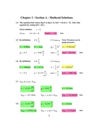
  • 1. Chapter 1 - Section A - Mathcad Solutions 1.4 The equation that relates deg F to deg C is: t(F) = 1.8 t(C) + 32. Solve this equation by setting t(F) = t(C). Guess solution: t t = 1.8t Given 0 Find t () 32 Ans. 40 P= 1.5 By definition: F A F = mass g A P 3000bar D 4mm F PA g 9.807 m D 4 F mass 2 g s P= 1.6 By definition: F A A 3000atm D 0.17in F PA g 32.174 ft 4 D mass 2 sec gh 13.535 1.8 gm 3 101.78kPa 13.535 g 9.832 mass 2 384.4 kg Ans. 2 F g A mass 2 0.023 in 1000.7 lbm Ans. gm 3 29.86in_Hg m h 2 56.38cm s Pabs g gh 32.243 Patm ft Pabs h 2 176.808 kPa Ans. 25.62in s cm Patm 12.566 mm Patm cm Patm A F = mass g P 1.7 Pabs = 2 Note: Pressures are in gauge pressure. Pabs gh 1 Patm Pabs 27.22 psia Ans.
  • 2. 1.10 Assume the following: 13.5 gm g 3 m 9.8 2 s cm P 1.11 P h 400bar h g Ans. 302.3 m The force on a spring is described by: F = Ks x where Ks is the spring constant. First calculate K based on the earth measurement then gMars based on spring measurement on Mars. On Earth: F = mass g = K x mass g 0.40kg 9.81 m x 2 1.08cm s F F mass g F x Ks 3.924 N Ks 363.333 N m On Mars: x 0.40cm gMars 1.12 Given: FMars gMars FMars mass d P= dz g 0.01 FMars Kx and: mK = 4 MP RT Substituting: Separating variables and integrating: 1 dP = P Psea 1atm ln M 29 2 mK PDenver Psea = PDenver = Psea e gm mol d P= dz zDenver Mg zDenver RT Mg zDenver RT g 9.8 MP g RT Mg dz RT 0 Psea Taking the exponential of both sides and rearranging: 3 Ans. kg PDenver After integrating: 10 m 2 s
  • 3. 3 R 82.06 cm atm T mol K Mg zDenver RT Mg RT ( 10 zDenver 273.15) K 0.194 zDenver Psea e PDenver 0.823 atm Ans. PDenver PDenver 1 mi 0.834 bar Ans. 1.13 The same proportionality applies as in Pb. 1.11. gearth ft 32.186 gmoon 2 5.32 M lmoon 1.14 gearth gmoon costbulb Ans. 18.767 lbf Ans. hr 0.1dollars 70W 10 day kW hr hr 5.00dollars 10 day 1000hr costelec dollars yr costelec 25.567 dollars yr costtotal 43.829 dollars yr Ans. 18.262 costtotal costbulb D 18.76 113.498 113.498 lbm wmoon M gmoon costbulb 1.15 learth M learth lbm wmoon lmoon 2 s s learth ft 1.25ft costelec mass 250lbm g 32.169 ft 2 s 3
  • 4. Patm (a) F 30.12in_Hg Patm A l Work 1.7ft D D 2 3 10 lbf Work PE mass g l mass 1.227 ft 2 Ans. Ans. 16.208 psia F l 0.47m A 2.8642 Pabs PE 1.16 4 F mass g F A (b) Pabs (c) A 3 10 ft lbf Ans. 4.8691 Ans. 424.9 ft lbf g 150kg 9.813 m 2 s Patm (a) F Patm A l 0.83m EP 1.18 mass EK 2 A 4 110.054 kPa Work EP mass g l u 1250kg 1 2 mass u 2 40 EK m s Work EK Wdot = 200W Ans. 1000 kJ mass g h 0.91 0.92 time Wdot Ans. 1000 kJ g 9.8 m 2 s 4 h 2 0.173 m Ans. 10 N F l Work 1.19 1.909 Pabs Work D 4 F mass g F A (b) Pabs (c) A 101.57kPa 50m Ans. 15.848 kJ Ans. 1.222 kJ Ans.
  • 5. Wdot mdot 1.22 a) cost_coal mdot g h 0.91 0.92 0.488 25.00 ton cost_coal MJ 29 kg cost_gasoline 0.95 GJ kg s 1 2.00 gal 37 GJ cost_gasoline Ans. 14.28 GJ 1 3 m cost_electricity 0.1000 kW hr cost_electricity 27.778 GJ 1 b) The electrical energy can directly be converted to other forms of energy whereas the coal and gasoline would typically need to be converted to heat and then into some other form of energy before being useful. The obvious advantage of coal is that it is cheap if it is used as a heat source. Otherwise it is messy to handle and bulky for tranport and storage. Gasoline is an important transportation fuel. It is more convenient to transport and store than coal. It can be used to generate electricity by burning it but the efficiency is limited. However, fuel cells are currently being developed which will allow for the conversion of gasoline to electricity by chemical means, a more efficient process. Electricity has the most uses though it is expensive. It is easy to transport but expensive to store. As a transportation fuel it is clean but batteries to store it on-board have limited capacity and are heavy. 5
  • 6. 1.24 Use the Matcad genfit function to fit the data to Antoine's equation. The genfit function requires the first derivatives of the function with respect to the parameters being fitted. B T C A Function being fit: f ( A B C) T e First derivative of the function with respect to parameter A d f ( A B C) T dA B exp A T C First derivative of the function with respect to parameter B d f ( A B C) T dB 1 T C B exp A T C First derivative of the function with respect to parameter C d f ( A B C) T dC B ( T 2 exp A C) 18.5 3.18 9.5 5.48 0.2 11.8 t 9.45 16.9 23.1 32.7 Psat 28.2 41.9 44.4 66.6 52.1 89.5 63.3 129 75.5 187 6 B T C
  • 7. T t 273.15 lnPsat ln ( ) Psat Array of functions used by Mathcad. In this case, a0 = A, a1 = B and a2 = C. exp a0 exp a0 F ( a) T a1 T a2 a1 T 1 exp a0 T a2 a1 T a2 2 Guess values of parameters 15 a2 guess a1 T exp a0 3000 50 a2 a1 T a2 Apply the genfit function A 13.421 A B B genfit ( Psat guess F) T C 2.29 C 3 10 Ans. 69.053 Compare fit with data. 200 150 Psat f ( A B C) T 100 50 0 240 260 280 300 320 340 360 T To find the normal boiling point, find the value of T for which Psat = 1 atm. 7
  • 8. Psat 1atm B Tnb A Tnb 1.25 a) t1 1970 C2 C1 ( 1 t2 i) 273.15K 2000 dollars gal C1 0.35 1.513 329.154 K Ans. 56.004 degC C2 t2 t1 Tnb C K Psat ln kPa i 5% dollars gal The increase in price of gasoline over this period kept pace with the rate of inflation. b) t1 1970 Given t2 C2 C1 = (1 2000 i) C1 t2 t1 i 16000 dollars yr Find ( i) i C2 80000 dollars yr 5.511 % The salary of a Ph. D. engineer over this period increased at a rate of 5.5%, slightly higher than the rate of inflation. c) This is an open-ended problem. The strategy depends on age of the child, and on such unpredictable items as possible financial aid, monies earned by the child, and length of time spent in earning a degree. 8
  • 9. Chapter 2 - Section A - Mathcad Solutions 2.1 (a) Mwt g 35 kg 9.8 m z 2 5m s Work (b) Work Mwt g z Utotal Utotal Work (c) By Eqs. (2.14) and (2.21): dU 1.715 kJ Ans. 1.715 kJ Ans. d ( )= CP dT PV Since P is constant, this can be written: MH2O CP dT = MH2O dU MH2O P dV Take Cp and V constant and integrate: MH2O CP t2 t1 = Utotal kJ MH2O 30 kg CP 4.18 t1 20 degC kg degC t2 t1 Utotal MH2O CP t2 20.014 degC Ans. (d) For the restoration process, the change in internal energy is equal but of opposite sign to that of the initial process. Thus Q (e) Utotal Q 1.715 kJ Ans. In all cases the total internal energy change of the universe is zero. 2.2 Similar to Pb. 2.1 with mass of water = 30 kg. Answers are: (a) W = 1.715 kJ (b) Internal energy change of the water = 1.429 kJ (c) Final temp. = 20.014 deg C (d) Q = -1.715 kJ 9
  • 10. 2.4 The electric power supplied to the motor must equal the work done by the motor plus the heat generated by the motor. E i 9.7amp Wdotelect Qdot 2.5 i E Wdotelect t Eq. (2.3): U = Q Step 1 to 2: Ut12 Wdotelect 1.067 3 134.875 W Ans. W W12 200J Ut12 Q34 Q12 800J Ut34 1.25hp 10 W Qdot Wdotmech Q12 Step 3 to 4: Wdotmech 110V W12 6000J W34 Q34 Ut34 W34 3 5.8 Ans. 10 J 300J Ans. 500 J t t Step 1 to 2 to 3 to 4 to 1: Since U is a state function, U for a series of steps that leads back to the initial state must be zero. Therefore, the sum of the t U values for all of the steps must sum to zero. Ut41 4700J Ut23 Step 2 to 3: Ut23 W23 Ut34 Ut41 Ans. 4000 J Ut23 Ut12 4 Ut23 3 Q23 Q23 3800J W23 10 J 200 J Ans. For a series of steps, the total work done is the sum of the work done for each step. W12341 1400J 10
  • 11. W41 W12341 Step 4 to 1: W12 W23 Ut41 Ut41 Ans. 10 J 3 4.5 Q41 W41 3 4.5 W41 4700J Q41 Note: W41 W34 10 J 200 J Ans. Q12341 = W12341 2.11 The enthalpy change of the water = work done. M Wdot 2.12 Q CP 20 kg 4.18 kJ kg degC t 10 degC M CP t 0.25 kW 0.929 hr Wdot Ans. U Q 12 kJ W U 19.5 kJ Ans. Q 12 kJ U W U 7.5 kJ Q 12 kJ Ans. 2.13Subscripts: c, casting; w, water; t, tank. Then mc Uc mw Uw mt Ut = 0 Let C represent specific heat, C = CP = CV Then by Eq. (2.18) mc Cc tc mw Cw tw mt Ct tt = 0 mc 2 kg mw Cc 0.50 kJ kg degC Ct mt 40 kg tc 500 degC Given t1 mc Cc t2 t2 0.5 5 kg kJ kg degC Cw 25 degC t2 30 degC tc = mw Cw mt Ct t2 Find t2 11 t2 4.18 kJ kg degC (guess) t1 27.78 degC Ans.
  • 12. 2.15 mass (a) (b) T g CV 1 kg Ut 1K 9.8 m Ut mass CV T EP 2 kJ kg K 4.18 Ans. 4.18 kJ Ut s z (c) 2.17 EP EK z z mass g 426.531 m Ans. EK u Ut 1 mass 2 1000 50m u kg 5 A 3 A 2m mdot Wdot uA mdot mdot g z Wdot 4 D 2 (b) 2 4 kg 1.571 10 7.697 s 3 10 kW U1 P1 1002.7 kPa U1 H1 763.131 U2 kJ 2784.4 kg H2 U2 P1 V 1 kJ kg kJ kg cm 1.128 gm V1 Ans. 3 P2 U P2 V 2 2022.4 Ans. 3 kJ 762.0 kg U Ans. 3.142 m H1 2.18 (a) m s m s u m D 91.433 Ans. 1500 kPa U2 U1 H 12 cm 169.7 gm V2 H 2275.8 kJ kg H2 H1 Ans.
  • 13. 2.22 D1 (a) u1 2.5cm m s D2 5cm For an incompressible fluid, =constant. By a mass balance, mdot = constant = u 1A1 = u2A2 u2 (b) D1 u1 u2 D2 1 EK 2 2 2 u2 1 2 2.23 Energy balance: Mass balance: u1 2 mdot3 H3 mdot1 1.0 Qdot 30 Qdot H1 T1 CP 4.18 s mdot1 mdot2 H2 = Qdot H2 = Qdot mdot2 CP T3 25degC kJ Ans. kg mdot2 H3 T1 kg s J mdot2 = 0 mdot2 = Qdot mdot1 CP T1 Ans. 1.875 mdot1 mdot Cp T3 T3 CP mdot1 m s mdot1 H1 mdot1 H3 or 0.5 EK mdot3 Therefore: T3 2 T2 = Qdot mdot1 CP T1 mdot2 CP T2 mdot2 0.8 kg s T2 75degC kJ kg K mdot2 CP T2 mdot2 CP T3 43.235 degC 2 2.25By Eq. (2.32a): By continuity, incompressibility H u = 0 2 A1 u2 = u1 13 A2 H = CP T CP 4.18 kJ kg degC Ans.
  • 14. 2 u = u1 u1 u1 2 2 CP D2 2 u = u1 1 m s 14 D1 D1 2 1 A2 SI units: T 2 A1 2 4 1 D2 D1 D2 2.5 cm 3.8 cm 4 T 0.019 degC Ans. T D2 0.023 degC Ans. 7.5cm u1 T 2 2 CP D1 1 4 D2 Maximum T change occurrs for infinite D2: D2 cm u1 T 2.26 T1 2 CP 300K Wsdot H 2 D1 1 T D2 T2 u1 520K ndot 98.8kW CP T2 4 50 H T1 10 0.023 degC m s u2 kmol hr 3.5 10 molwt 29 kg kmol 7 R 2 CP 6.402 m s Ans. 3 kJ kmol By Eq. (2.30): Qdot H 2 u2 2 2 u1 2 molwt ndot Wsdot Qdot 2 2.27By Eq. (2.32b): By continunity, constant area H= u2 = u1 u 2 gc V2 u2 = u1 V1 14 also T 2 P1 T 1 P2 Ans. 9.904 kW V2 V1 = 2 T 2 P1 T 1 P2 2 u = u2 u1 2
  • 15. 2 u = u1 P1 R T2 T2 P2 molwt mol rankine 7 2 u1 20 psi ft lbf 28 20 7 R T2 2 ft s T1 T1 579.67 rankine H2 2726.5 kJ kg kJ kg Ans. gm mol (guess) 578 rankine Given H = CP T = 1 T 1 P2 100 psi 3.407 2 T 2 P1 2 2 R T2 T1 = T2 Find T2 u1 2 2 T 2 P1 T 1 P2 1 molwt Ans. 578.9 rankine ( 119.15 degF) 2.28 u1 3 m s u2 200 m s H1 2 By Eq. (2.32a): 2.29 u1 u2 m s m 500 s 30 By Eq. (2.32a): Q H2 H1 3112.5 u1 u2 H1 334.9 kJ kg 2 Q 2 kJ H2 kg 2411.6 2945.7 (guess) 2 H2 Given u2 578.36 m s H1 = u2 u1 2 5 cm V1 388.61 u2 2 Ans. 3 3 D1 kJ kg cm gm 15 V2 667.75 cm gm Find u2
  • 16. Continuity: 2.30 (a) t1 D2 t2 30 degC CV u1 V2 u2 V1 D1 D2 Ans. 1.493 cm n 250 degC 3 mol J mol degC 20.8 By Eq. (2.19): Q n CV t2 Q t1 Ans. 13.728 kJ Take into account the heat capacity of the vessel; then cv mv Q (b) 100 kg mv cv t1 200 degC CP 29.1 n CV CV Q Q Ans. 11014 kJ n 40 degC 4 mol joule mol degC Q n CP t2 t2 70 degF 5 kJ kg degC t1 t2 By Eq. (2.23): 2.31 (a) t1 t2 0.5 BTU mol degF n CV t2 Q t1 18.62 kJ n 350 degF 3 mol By Eq. (2.19): Q t1 4200 BTU Ans. Take account of the heat capacity of the vessel: mv Q mv cv cv 200 lbm (b) t1 400 degF n CV t2 0.12 BTU lbm degF Q t1 t2 150 degF 16 10920 BTU n Ans. 4 mol Ans.
  • 17. CP 7 BTU mol degF Q H1 2.33 n CP t2 1322.6 V1 Q t1 BTU BTU lbm 1148.6 3 V2 lbm 78.14 ft 4 mdot mdot V2 10 22.997 u2 Wdot 2.34 H1 V1 H2 307 9.25 BTU lbm ft H2 330 V2 u1 lbm ft 0.28 173.99 BTU lb Ans. 39.52 hp BTU 3 lbm Ws 2 Wdot Ws mdot u1 u2 H1 20 ft s molwt 44 3 D1 lbm D2 4 in 1 in 2 mdot u2 4 D1 u1 mdot V1 V2 mdot u2 679.263 9.686 2 4 D2 2 Eq. (2.32a): Q H2 H1 10 in sec 2 D2 Eq. (2.32a): Ws D2 ft sec 2 4 3 in 4 lb 3.463 V1 mdot 10 D1 lbm 2 u2 ft s u1 3 2 D 1 u1 Ans. 7000 BTU H2 lbm ft 3.058 By Eq. (2.23): ft sec u1 u2 2 17 lb hr 2 Ws Ws molwt 5360 Q BTU lbmol 98.82 BTU lbm gm mol
  • 18. Qdot 2.36 T1 Qdot mdot Q P 300 K 67128 BTU hr Ans. 1 kg n 1 bar 28.9 V1 n gm 34.602 mol mol 3 3 bar cm T1 83.14 mol K P cm 24942 mol V1 V2 P dV = n P V 1 W= n V2 = n P V1 3 V1 V1 Whence W Given: V2 V1 joule 29 Q n H U mol K Q = T1 3 Whence T1 Q W U n CP T2 602.08 kJ 12.41 kJ mol Ans. 172.61 kJ H T2 = T1 CP W n P 2 V1 T2 H 3 T1 17.4 kJ mol Ans. Ans. Ans. 2.37 Work exactly like Ex. 2.10: 2 steps, (a) & (b). A value is required for PV/T, namely R. R 8.314 T1 (a) Cool at const V1 to P2 (b) Heat at const P2 to T2 Ta2 T1 P2 P1 Ta2 293.15 K T2 333.15 K P1 J mol K 1000 kPa P2 100 kPa 7 R 2 CP 29.315 K 18 CV 5 R 2
  • 19. Tb T2 Hb C P Tb Hb Ua CV Ta Ua R T1 V1 P1 Ta2 Tb V1 303.835 K 2.437 8.841 Ta 10 5.484 10 mol Ha Ua V 1 P2 P1 Ha Ub Hb P2 V 2 V1 Ub U Ub U 0.831 H 2.39 Ua Ha Hb H 1.164 996 kg 9.0 10 3 D 5 2 kJ mol ms 1 cm u 5 1 m 5 s 5 22133 Re D u Re Ta 263.835 K mol 3 J mol V2 3 R T2 V2 P2 7.677 6.315 0.028 m mol 3 J 10 mol 3 J 10 mol Ans. mol 4 kg m 2 kJ T1 3 J 3 3 m 10 Ta2 55333 110667 276667 19 Ans. D 0.0001 Note: D = /D in this solution
  • 20. 0.00635 fF 0.3305 ln 0.27 D 7 Re 0.9 2 0.00517 fF 0.00452 0.0039 0.313 mdot u 4 D 2 mdot 1.956 kg 1.565 s Ans. 9.778 0.632 P L 2 fF D 2 P L u 0.206 kPa 11.254 m Ans. 3.88 2.42 mdot 4.5 kg s H1 761.1 kJ kg H2 536.9 kJ kg Assume that the compressor is adiabatic (Qdot = 0). Neglect changes in KE and PE. Wdot Cost mdot H2 15200 H1 Wdot Wdot 1.009 3 10 kW 0.573 Cost kW 20 799924 dollars Ans.
  • 21. Chapter 3 - Section A - Mathcad Solutions 3.1 1 d = 1 = dT d dP P T At constant T, the 2nd equation can be written: d = 2 ln dP 6 44.1810 P = 1 bar 2 = 1.01 1 ln ( ) 1.01 P P Ans. P2 = 226.2 bar 225.2 bar 3 3.4 b cm 0.125 gm c 2700 bar P1 P2 1 bar 500 bar V2 Since Work = a bit of algebra leads to P dV V1 P2 Work c P P b dP Work 0.516 Work 0.516 P1 J Ans. gm Alternatively, formal integration leads to Work 3.5 = a P1 c P2 P1 a bP P2 1 atm b ln P2 b P1 b 3.9 10 6 atm 1 b V 3000 atm 0.1 10 1 ft 3 9 J gm Ans. atm 2 (assume const.) Combine Eqs. (1.3) and (3.3) for const. T: P2 Work ( a V Work b P)P dP P1 21 16.65 atm ft 3 Ans. 1
  • 22. 3.6 1.2 10 V1 3 degC 1 CP 0.84 kJ kg degC M 5 kg t2 20 degC 3 m 1 P 1590 kg t1 1 bar 0 degC With beta independent of T and with P=constant, dV = V V2 dT Vtotal Vtotal M V Work V1 exp P Vtotal M CP t2 P2 (a) Constant V: T2 T1 U H R T1 ln (c) Adiabatic: T1 P1 Ans. 84 kJ 84 kJ Ans. 83.99 kJ Ans. T T1 U 10.91 15.28 H= 0 Q= 0 22 kJ mol kJ mol Work and CV U = Q = CV T T2 and 7 R 2 CP 600 K and Q Ans. Utotal U= P2 7.638 joule Work H CP T (b) Constant T: Work Q 1 bar V1 Ans. Q Q and CV T m t1 T P1 3 V2 Htotal W= 0 P2 10 Q Utotal 8 bar 5 V Work 7.638 Htotal P1 t1 (Const. P) Q 3.8 t2 525 K Ans. Ans. and 10.37 Q= W kJ mol Ans. U = W = CV T 5 2 R
  • 23. 1 CP T2 CV P2 T1 U and U 5.586 3.9 P4 2bar CP H kJ 7 R 2 10bar T1 Step 41: Adiabatic T 331.227 K Ans. mol T4 R T1 P1 V1 P4 T1 kJ mol Ans. 5 R 2 CV 600K 7.821 T2 CP T H CV T W P1 T2 P1 V1 4.988 T4 3 3 m 10 378.831 K mol R CP P1 3 J U41 CV T1 T4 U41 4.597 10 H41 CP T1 T4 H41 6.436 10 Q41 3bar T2 Step 12: Isothermal Q41 U41 W41 4.597 mol J 0 mol W41 P2 J 0 mol mol 3 J V2 600K U12 0 J mol H12 0 J mol 23 R T2 P2 3 J 10 3 V2 m 0.017 mol U12 0 J mol H12 0 J mol mol T1
  • 24. Q12 W12 P3 2bar V3 Q12 Q12 P1 W12 P3 V 3 T3 V2 Step 23: Isochoric P2 R T1 ln T3 R U23 CV T3 H23 CP T3 T2 Q23 2 bar T4 CV T3 W23 P4 0 T2 R T4 V4 3 J 10 mol 3 J 6.006 10 400 K 3 J 4.157 10 P4 3 V4 m 0.016 mol U34 CV T4 T3 U34 439.997 H34 CP T4 T3 H34 615.996 Q34 CP T4 T3 Q34 W34 R T4 T3 W34 3.10 For all parts of this problem: T2 = T1 mol mol 3 J H23 5.82 10 mol 3 J Q23 4.157 10 mol J W23 0 mol J mol 378.831 K Step 34: Isobaric U23 T2 6.006 615.996 175.999 J mol J mol J mol J mol and Also Q = Work and all that remains is U= H= 0 to calculate Work. Symbol V is used for total volume in this problem. P1 1 bar P2 V1 12 bar 24 3 12 m V2 3 1m
  • 25. (a) P2 Work = n R T ln Work P1 Work P1 V1 ln P2 P1 Ans. 2982 kJ (b) Step 1: adiabatic compression to P2 1 5 3 Vi P2 V i W1 V1 P1 P2 (intermediate V) P1 V 1 Vi W1 3063 kJ W2 1 3 2.702 m 2042 kJ Step 2: cool at const P2 to V2 W2 P2 V 2 Work W1 Vi W2 Work 5106 kJ Ans. (c) Step 1: adiabatic compression to V2 Pi W1 P1 V1 (intermediate P) V2 Pi V 2 1 Step 2: No work. Work (d) Step 1: heat at const V1 to P2 62.898 bar W1 P1 V 1 Pi 7635 kJ W1 Work 7635 kJ Ans. W2 Work 13200 kJ Ans. W1 = 0 Step 2: cool at const P2 to V2 W2 P2 V 2 V1 Work (e) Step 1: cool at const P1 to V2 W1 P1 V 2 W1 V1 25 1100 kJ
  • 26. Step 2: heat at const V2 to P2 Work 3.17(a) W2 = 0 Work W1 No work is done; no heat is transferred. t U = (b) T= 0 Not reversible T2 = T1 = 100 degC The gas is returned to its initial state by isothermal compression. Work = n R T ln 3 V1 3.18 (a) P1 P2 V2 ln 7 2 but V2 4 3 3 P2 V1 6 bar 878.9 kJ Ans. Work V2 T1 500 kPa 303.15 K CP 5 R 2 CV R n R T = P2 V 2 m P2 100 kPa CP V1 V2 4m Work CV Adiabatic compression from point 1 to point 2: Q12 0 kJ mol 1 U12 = W12 = CV T12 U12 CV T2 U12 3.679 T1 kJ mol T2 H12 CP T2 W12 H12 5.15 T1 kJ W12 mol T1 3.679 P2 P1 U12 kJ mol Cool at P2 from point 2 to point 3: T3 Ans. 1100 kJ H23 T1 U23 CV T3 CP T3 W23 T2 26 Q23 T2 U23 Q23 H23 Ans.
  • 27. H23 5.15 Q23 5.15 kJ U23 mol kJ W23 mol kJ mol 3.679 Ans. kJ 1.471 Ans. mol Isothermal expansion from point 3 to point 1: U31 = H31 = 0 Q31 4.056 W31 P2 P1 R T3 ln P3 W31 W31 P3 kJ mol FOR THE CYCLE: Q Q Q12 1.094 Q23 Q31 U= 4.056 kJ mol Ans. H= 0 Work kJ mol W12 Work Q31 1.094 W23 W31 kJ mol (b) If each step that is 80% efficient accomplishes the same change of state, all property values are unchanged, and the delta H and delta U values are the same as in part (a). However, the Q and W values change. Step 12: W12 Q12 Step 23: W23 Q23 Step 31: W31 Q31 W12 W12 W23 0.8 U23 4.598 Q12 0.92 kJ mol W23 0.8 U12 kJ W12 1.839 kJ mol mol W31 0.8 W31 Q23 5.518 kJ mol W31 W23 3.245 kJ mol Q31 27 3.245 kJ mol
  • 28. FOR THE CYCLE: Q Q12 Q Q23 3.192 Work kJ mol W12 Work Q31 3.192 W23 W31 kJ mol 3.19Here, V represents total volume. P1 CP 21 CV joule mol K CP T2 208.96 K P1 V 1 n P1 V 1 T2 Work n CV P2 P1 V2 Ans. T1 P2 V 2 P1 V 1 69.65 kPa Ans. Work Work = Work Pext V2 994.4 kJ Ans, U = Pext V V1 Work U = n CV T R T1 V1 Ans. 1609 kJ V2 P2 P1 200 kPa T2 1 100 kPa V2 V1 P1 (c) Restrained adiabatic: Pext P2 Work P2 P2 V 2 V1 P2 600 K T2 Work CV V2 (b) Adiabatic: 600 K CP V1 P1 V1 ln T1 5 V1 R Work = n R T1 ln T1 Work V2 1m (a) Isothermal: T2 3 V1 1000 kPa T2 V 1 T2 V 2 T1 28 442.71 K Ans. P2 T1 147.57 kPa Ans. 400 kJ Ans.
  • 29. 3.20 T1 CP P1 423.15 K 7 2 Step 12: If V1 V2 = 2.502 Step 23: V1 V3 kJ mol 0 Process: 2.079 U12 mol mol R T1 ln r () Q12 2.502 CV T3 CP T3 T2 2.079 W23 kJ mol H23 Work Q Q23 2.502 0.424 2.91 kJ mol kJ mol kJ mol H H12 H23 H 2.91 U U12 U23 U 2.079 29 kJ mol T2 H23 W12 Q12 kJ U23 U23 Q 323.15 K W12 W12 U23 Work 0 T 3 P1 kJ mol kJ mol T3 T 1 P3 r Q12 W23 T1 kJ Then Q23 Q23 0 3 bar T2 R 2 H12 r= W12 5 CV R P3 8bar kJ mol kJ mol Ans. Ans. Ans. Ans.
  • 30. 3.21 By Eq. (2.32a), unit-mass basis: But CP u1 2.5 t2 3.22 28 Whence H = CP T R 7 2 molwt molwt u2 1 2 H u2 T= m s u2 t1 gm mol 2 2 u1 2 CP 50 m s t1 u1 t2 2 CP 7 R 2 CV 5 R 2 P1 1 bar P3 148.8 degC Ans. 10 bar CV T3 U 2.079 T1 mol CP T3 H Ans. T3 303.15 K H T1 kJ 2.91 T1 kJ mol Each part consists of two steps, 12 & 23. (a) T2 W23 T3 R T2 ln P2 P3 P2 P1 150 degC 2 2 CP U 2 u = 0 T2 T1 Work W23 Work 6.762 Q U Q 4.684 30 kJ mol Ans. Work kJ mol Ans. Ans. 403.15 K
  • 31. (b) P2 T2 P1 H12 CP T2 W12 U12 W23 R T2 ln Work W12 Q (c) U T2 U12 T3 CV T2 Q12 Q12 P3 H12 W12 T1 0.831 W23 P2 Work W23 Q Work P2 T1 P3 T1 W12 kJ mol 7.718 6.886 4.808 kJ mol kJ mol kJ mol CP T3 T2 Q23 CV T3 T2 W23 U23 Work 4.972 P1 H23 U23 Ans. P2 R T1 ln H23 Ans. Work Q W12 U W23 Q Work 2.894 Q23 kJ mol kJ mol For the second set of heat-capacity values, answers are (kJ/mol): U = 2.079 U = 1.247 (a) Work = 6.762 Q = 5.515 (b) Work = 6.886 Q = 5.639 (c) Work = 4.972 Q = 3.725 31 Ans. Ans.
  • 32. 3.23 T1 303.15 K T2 T1 T3 393.15 K P1 1 bar P3 12 bar CP 7 R 2 For the process: U U Step 12: W12 CV T3 1.871 P2 5.608 kJ mol mol For the process: Work W12 Q 3.24 Work 5.608 W12 = 0 Work = W23 = P2 V3 But T3 = T1 Also W = R T1 ln ln P T2 T1 P = P1 T1 P1 exp T2 T2 R T1 ln 5.608 P P1 Ans. P2 U P1 kJ mol W23 kJ Q mol 3.737 V 2 = R T3 kJ mol Ans. T2 Work = R T2 So... mol Q23 kJ mol W23 Q23 kJ Q12 W12 Step 23: Q12 2.619 T1 W12 T3 0 CP T3 H kJ T1 P3 Q12 H T1 5 R 2 CV T1 Therefore T1 T1 32 T1 800 K P 350 K 2.279 bar P1 Ans. 4 bar
  • 33. 3.25 3 VA P Define: 256 cm P1 r 0.0639 VB 3750.3 cm CV = r CP Assume ideal gas; let V represent total volume: P1 V B = P 2 V A P P1 3.26 T1 = VA VA VA ( 1) r VB VB 300 K From this one finds: VB P1 r 1 atm CP 7 R 2 3 Ans. CP R CV The process occurring in section B is a reversible, adiabatic compression. Let TA ( )= TA final P ( )= P2 final TB ( )= TB final Since the total volume is constant, nA = nB nA R TA 2 nA R T1 = P2 P1 TB TA TB 2 T1 = P2 P1 or (1) 1 (a) P2 TA 2 T1 TB 1.25 atm P2 P1 Q = nA TB Define q= TB TA 319.75 K T1 Q nA q 430.25 K 33 P2 (2) P1 UA CV TA q UB TB 2 T1 3.118 kJ mol (3) Ans.
  • 34. (b) Combine Eqs. (1) & (2) to eliminate the ratio of pressures: (guess) 425 K TB 300 K TB Find TB TB TA 319.02 K Ans. P2 1.24 atm Ans. kJ mol Ans. 1 TB = T1 Given P2 P1 q (c) TA P1 TA 2 T1 P2 P2 (1) TB P1 kJ mol 2.993 1 T1 CV TA 3 q 2 T1 By Eq. (2), TB Eliminate q (1) TB TB P2 (d) 2 T1 TB 325 K q TB 2 T1 CV TA TB TA Ans. TA 469 K Ans. q 2 T1 TA 1.323 atm TB q P1 2 T1 C V 4.032 kJ mol Ans. from Eqs. (1) & (3): P2 1.241 atm Ans. (2) P2 TB 319.06 K Ans. (1) TA 425.28 K Ans. P1 1 TB T1 TA 2 T1 P2 P1 P2 P1 TB 34
  • 35. 6 3 3.30 B P1 B' cm 242.5 C 25200 mol mol P2 7.817 T B C 10 3 1 bar B 2 373.15 K 2 55 bar B' 1 bar RT C' cm R T 2 C' 2 3.492 10 5 1 2 bar (a) Solve virial eqn. for initial V. RT P1 Guess: V1 Given P1 V 1 = 1 RT B V1 3 C V1 2 V1 V2 Find V1 cm 30780 mol cm 241.33 mol V1 Solve virial eqn. for final V. Guess: RT P2 V2 P2 V 2 Given RT = 1 B V2 3 C V2 2 V2 Find V2 Eliminate P from Eq. (1.3) by the virial equation: V2 Work RT 1 B V C V 2 1 dV V Work 12.62 kJ mol V1 (b) Eliminate dV from Eq. (1.3) by the virial equation in P: P2 1 dV = R T P C' dP W 1 P RT 2 P1 W 35 12.596 kJ mol Ans. C' P dP Ans.
  • 36. Note: The answers to (a) & (b) differ because the relations between the two sets of parameters are exact only for infinite series. 3.32 Tc 282.3 K T 298.15 K Pc 50.4 bar P 12 bar T Tc Tr Pr Tr Pr P Pc 6 3 B Given cm 140 C mol PV = 1 RT 7200 cm mol B V V (b) B0 V Find ( ) V Tr V Tr Z 1 (c) B0 cm 1919 mol B1 B1 4.2 Tr Z PV RT Z B0 1.6 Pr 3 V 2066 cm mol 2 0.172 0.139 RT P C 0.422 0.083 V 2 3 B1 0.238 (guess) 0.087 (a) 1.056 Ans. Z 0.929 V cm Ans. 1924 mol 0.304 2.262 0.932 10 V 3 3 ZRT P For Redlich/Kwong EOS: 0 1 ( ) Tr T r Pr Tr 0.5 Pr Tr Table 3.1 Eq. (3.53) 36 Table 3.1 0.42748 0.08664 q Tr Tr Tr Eq. (3.54)
  • 37. Calculate Z Guess: Given T r Pr 0.9 Eq. (3.52) Z= 1 Z Z Z Find Z) ( (d) q Tr Z T r Pr Z T r Pr Z T r Pr 3 Z RT V 0.928 T r Pr V P 1916.5 cm mol Ans. For SRK EOS: 2 1 Tr 1 0.480 Tr q Tr (e) 1 Tr Guess: Z Table 3.1 2 Pr T r Pr Tr T r Pr q Tr Z Find Z) ( 0.9 Z T r Pr Z V 0.928 T r Pr T r Pr Z T r Pr 3 Z RT V P 1918 1 2 0.45724 0.07779 2 1 q Tr cm mol Ans. For Peng/Robinson EOS: 1 Tr Eq. (3.53) Tr Eq. (3.52) Given Z 0.176 Eq. (3.54) Calculate Z Z= 1 1.574 2 Table 3.1 0.42748 0.08664 0 1 1 0.37464 Tr 1.54226 0.26992 Eq. (3.54) Tr 37 2 T r Pr 1 Tr Pr Tr 2 Table 3.1 2 Table 3.1 Eq. (3.53)
  • 38. Calculate Z Guess: 0.9 Eq. (3.52) Given Z= 1 T r Pr Z Z Find ( Z) q Tr Z Z T r Pr Z T r Pr 3 V 1900.6 cm mol 305.3 K Pc T 323.15 K Tr T Tc Tr P 15 bar Pr P Pc Pr 0.308 (guess) 0.100 6 3 (a) cm 156.7 mol B Given PV = 1 RT B V C 9650 cm mol V (b) B0 V Find ( V) Tr B1 V Tr (c) B0 cm 1625 mol B1 B1 4.2 Tr Z PV Z B0 1.6 Pr 3 V cm 1791 mol 2 0.172 0.139 RT P C 0.422 0.083 V 2 3 1 Ans. 1.058 48.72 bar 3.33 Tc Z Z T r Pr ZRT P V 0.92 T r Pr Ans. Z RT 0.907 V cm Ans. 1634 mol 0.302 3.517 0.912 V 10 3 ZRT P 3 For Redlich/Kwong EOS: 1 0 0.08664 38 0.42748 Table 3.1
  • 39. ( ) Tr 0.5 Tr Table 3.1 Pr T r Pr Tr q Tr Eq. (3.54) Tr Eq. (3.53) Tr Calculate Z Guess: Given T r Pr 0.9 Eq. (3.52) Z= 1 Z Z Z Find Z) ( (d) q Tr Z T r Pr Z Z T r Pr cm 1622.7 mol V P Ans. For SRK EOS: 0.42748 0.08664 0 1 Tr 1 0.480 Tr q Tr 0.176 Eq. (3.54) Guess: 2 1 Tr T r Pr Tr Calculate Z Z Table 3.1 2 Pr Eq. (3.53) Tr 0.9 Eq. (3.52) Given Z= 1 Z 1.574 Table 3.1 2 1 (e) T r Pr 3 Z RT V 0.906 T r Pr T r Pr Find Z) ( q Tr Z T r Pr Z Z V 0.907 T r Pr Z RT P T r Pr Z T r Pr 3 V 1624.8 cm mol Ans. For Peng/Robinson EOS: 1 2 1 0.07779 2 39 0.45724 Table 3.1
  • 40. 1 Tr 1 0.37464 Tr q Tr 1.54226 0.26992 Eq. (3.54) 1 Guess: Z Tr Table 3.1 2 Pr T r Pr Tr Calculate Z 2 2 Eq. (3.53) Tr 0.9 Eq. (3.52) Given Z= 1 T r Pr q Tr Z Z T r Pr Z T r Pr Z T r Pr 3 ZRT V 0.896 T r Pr cm 1605.5 mol V Z Find ( Z) 3.34 Tc 318.7 K T 348.15 K Tr T Tc Tr Pc 37.6 bar P 15 bar Pr P Pc Pr Ans. 1.092 0.399 P 0.286 (guess) 6 3 (a) B Given 194 cm C mol PV = 1 RT 15300 cm mol B V V cm 1722 mol Find ( V) (b) B0 0.083 V 1930 mol 2 3 V 3 cm C V V 2 RT P 0.422 Tr 1.6 B0 40 Z 0.283 PV RT Z 0.893 Ans.
  • 41. B1 0.172 0.139 Tr Z 1 B0 (c) B1 4.2 Pr B1 Z Tr 0.02 V 0.899 3 Z RT V P 1734 cm mol Ans. For Redlich/Kwong EOS: ( ) Tr Tr 0.5 Table 3.1 Pr T r Pr Table 3.1 0.42748 0.08664 0 1 Tr q Tr Eq. (3.54) Tr Eq. (3.53) Tr Calculate Z Guess: Given T r Pr 0.9 Eq. (3.52) Z= 1 Z Z Find Z) ( (d) q Tr Z Z T r Pr Z T r Pr Z T r Pr 3 Z RT V 0.888 T r Pr cm 1714.1 mol V P Ans. For SRK EOS: 0.42748 0.08664 0 1 1 Tr q Tr 1 0.480 Tr 1.574 0.176 Eq. (3.54) Tr 41 2 1 T r Pr Tr Table 3.1 2 Table 3.1 2 Pr Tr Eq. (3.53)
  • 42. Calculate Z Guess: Eq. (3.52) Given Z= 1 T r Pr Z (e) q Tr Z Find ( Z) Z 0.9 Z T r Pr Z Z T r Pr T r Pr 3 ZRT P V 0.895 T r Pr V 1726.9 Ans. mol For Peng/Robinson EOS: 1 1 2 0.45724 0.07779 2 1 Tr 1 0.37464 Tr q Tr T r Pr Guess: Z T r Pr q Tr Z Find ( Z) Tr 2 Table 3.1 2 Pr Eq. (3.53) Tr 0.9 523.15 K Z T r Pr Z ZRT P V 0.882 P T r Pr cm 152.5 mol B Given Z PV RT T r Pr Z T r Pr 3 cm 1701.5 mol V Ans. 1800 kPa 6 3 (a) 1 Table 3.1 Eq. (3.52) Z= 1 T 2 0.26992 Tr Given Z 1.54226 Eq. (3.54) Calculate Z 3.35 cm C mol C B V PV = 1 RT V 2 2 V RT (guess) P V 5800 cm Find ( V) 3 V 2250 42 cm mol Z 0.931 Ans.
  • 43. (b) Tc Tr Tr B1 647.1 K Pc T Tc Pr 0.139 0.172 Tr (c) Table F.2: B0 Pc 4.2 0.422 0.083 Tr B0 0.082 B1 0.51 Z 0.281 1.6 1 B0 B1 Pr Tr 3 Z RT P V P Pr 0.808 0.345 220.55 bar Z molwt V V cm molwt 124.99 gm V 0.939 cm 2268 mol cm 2252 mol Ans. 3 gm 18.015 mol 3 or cm 53.4 mol B T Zi Z1i C 2620 cm mol 2 D 5000 cm mol 3 n mol 273.15 K PV Given i 9 6 3 3.37 Ans. RT 0 10 Pi fPi Vi Pi RT 1 B Pi RT = 1 10 B V 10 C V 2 D V fP V) ( 3 RT Pi Vi 20 i bar Find V) ( (guess) Eq. (3.12) Eq. (3.38) 43 Z2i 1 2 1 4 B Pi RT Eq. (3.39)
  • 45. 3.38 (a) Propane: Tc Tc 313.15 K P Tr T Pc T Tr 369.8 K 0.847 Pr 0.152 42.48 bar 13.71 bar P Pc Pr 0.323 For Redlich/Kwong EOS: ( ) Tr Tr 0.5 Table 3.1 Pr T r Pr Table 3.1 0.42748 0.08664 0 1 Tr q Tr Eq. (3.54) Tr Eq. (3.53) Tr Calculate Z for liquid by Eq. (3.56) Guess: Z 0.01 Given Z= Z T r Pr Z Find Z) Z ( T r Pr 0.057 Z Calculate Z for vapor by Eq. (3.52) Z T r Pr q Tr T r Pr 3 Z RT P V 1 T r Pr V Guess: 108.1 cm Ans. mol Z 0.9 V cm 1499.2 mol Given Z= 1 Z T r Pr Find Z) ( q Tr Z T r Pr Z Z Z V 0.789 45 T r Pr T r Pr Z RT P 3 Ans.
  • 46. Rackett equation for saturated liquid: T Tc Tr Tr 0.847 3 Vc V 200.0 V c Zc cm Zc mol 1 Tr 0.276 3 0.2857 V 94.17 cm Ans. mol For saturated vapor, use Pitzer correlation: B0 0.083 0.422 Tr B1 0.139 V 0.468 B1 0.207 0.172 Tr RT P B0 1.6 4.2 R B0 B1 Tc V Pc 46 1.538 3 3 cm 10 mol Ans.
  • 47. Parts (b) through (t) are worked exactly the same way. All results are summarized as follows. Volume units are cu.cm./mole. R/K, Liq. R/K, Vap. Rackett Pitzer (a) 108.1 1499.2 94.2 1537.8 (b) 114.5 1174.7 98.1 1228.7 (c) 122.7 920.3 102.8 990.4 (d) 133.6 717.0 109.0 805.0 (e) 148.9 1516.2 125.4 1577.0 (f) 158.3 1216.1 130.7 1296.8 (g) 170.4 971.1 137.4 1074.0 (h) 187.1 768.8 146.4 896.0 (i) 153.2 1330.3 133.9 1405.7 (j) 164.2 1057.9 140.3 1154.3 (k) 179.1 835.3 148.6 955.4 (l) 201.4 645.8 160.6 795.8 (m) 61.7 1252.5 53.5 1276.9 (n) 64.1 1006.9 55.1 1038.5 (o) 66.9 814.5 57.0 853.4 (p) 70.3 661.2 59.1 707.8 (q) 64.4 1318.7 54.6 1319.0 (r) 67.4 1046.6 56.3 1057.2 (s) 70.8 835.6 58.3 856.4 (t) 74.8 669.5 60.6 700.5 47
  • 48. 3.39 (a) Propane T Tc 273.15)K T Tr ( 40 T Tc Tr Pc 369.8 K Pr 0.847 0.152 42.48 bar P P Pc 13.71 bar Pr 313.15 K 0.323 From Table 3.1 for SRK: 0.42748 0.08664 0 1 2 1 Tr 1 0.480 Tr q Tr 1.574 0.176 Eq. (3.54) 2 1 2 Tr Pr T r Pr Tr Calculate Z for liquid by Eq. (3.56) Guess: Eq. (3.53) Tr Z 0.01 Given Z= Z T r Pr Find Z) ( Z Z T r Pr 0.055 Z Calculate Z for vapor by Eq. (3.52) Z T r Pr q Tr T r Pr 3 Z RT P V 1 T r Pr cm 104.7 mol V Guess: Z Ans. 0.9 Given Z= 1 Z T r Pr Find Z) ( q Tr Z 0.78 Z T r Pr Z V 48 T r Pr Z T r Pr Z RT P T r Pr 3 V 1480.7 cm mol Ans.
  • 49. Parts (b) through (t) are worked exactly the same way. All results are summarized as follows. Volume units are cu.cm./mole. SRK, Liq. SRK, Vap. Rackett Pitzer (a) 104.7 1480.7 94.2 1537.8 (b) 110.6 1157.8 98.1 1228.7 (c) 118.2 904.9 102.8 990.4 (d) 128.5 703.3 109.0 805.0 (e) 142.1 1487.1 125.4 1577.0 (f) 150.7 1189.9 130.7 1296.8 (g) 161.8 947.8 137.4 1074.0 (h) 177.1 747.8 146.4 896.0 (i) 146.7 1305.3 133.9 1405.7 (j) 156.9 1035.2 140.3 1154.3 (k) 170.7 815.1 148.6 955.4 (l) 191.3 628.5 160.6 795.8 (m) 61.2 1248.9 53.5 1276.9 (n) 63.5 1003.2 55.1 1038.5 (o) 66.3 810.7 57.0 853.4 (p) 69.5 657.4 59.1 707.8 (q) 61.4 1296.8 54.6 1319.0 (r) 63.9 1026.3 56.3 1057.2 (s) 66.9 817.0 58.3 856.4 (t) 70.5 652.5 60.6 700.5 49
  • 50. 3.40 (a) Propane T ( 40 Tr Tc T Tc Pc 369.8 K T 273.15)K Tr P P Pc 13.71 bar Pr 313.15 K Pr 0.847 0.152 42.48 bar 0.323 From Table 3.1 for PR: 2 1 Tr 1 1 0.37464 1 2 0.26992 2 Eq. (3.54) 1 2 Pr T r Pr Tr Tr 0.45724 0.07779 2 Tr q Tr 1.54226 Calculate Z for liquid by Eq. (3.56) Guess: Eq. (3.53) Tr Z 0.01 Given Z= Z T r Pr Find Z) ( Z Z T r Pr 0.049 Z Calculate Z for vapor by Eq. (3.52) Z T r Pr q Tr T r Pr 3 Z RT P V 1 T r Pr cm 92.2 mol V Guess: Z Ans. 0.6 Given Z= 1 Z T r Pr Find Z) ( q Tr Z 0.766 Z T r Pr Z V 50 T r Pr Z T r Pr Z RT P T r Pr 3 V 1454.5 cm mol Ans.
  • 51. Parts (b) through (t) are worked exactly the same way. All results are summarized as follows. Volume units are cu.cm./mole. PR, Liq. PR, Vap. Rackett Pitzer (a) 92.2 1454.5 94.2 1537.8 (b) 97.6 1131.8 98.1 1228.7 (c) 104.4 879.2 102.8 990.4 (d) 113.7 678.1 109.0 805.0 (e) 125.2 1453.5 125.4 1577.0 (f) 132.9 1156.3 130.7 1296.8 (g) 143.0 915.0 137.4 1074.0 (h) 157.1 715.8 146.4 896.0 (i) 129.4 1271.9 133.9 1405.7 (j) 138.6 1002.3 140.3 1154.3 (k) 151.2 782.8 148.6 955.4 (l) 170.2 597.3 160.6 795.8 (m) 54.0 1233.0 (n) 56.0 987.3 55.1 1038.5 (o) 58.4 794.8 57.0 853.4 (p) 61.4 641.6 59.1 707.8 (q) 54.1 1280.2 54.6 1319.0 (r) 56.3 1009.7 56.3 1057.2 (s) 58.9 800.5 58.3 856.4 (t) 62.2 636.1 60.6 700.5 53.5 1276.9 51
  • 52. 3.41 (a) For ethylene, molwt 28.054 gm Tc mol 282.3 K Pc 50.40 bar 0.087 T Tr Tc 328.15 K P 35 bar P Pc Pr T Tr 1.162 Pr 0.694 From Tables E.1 & E.2: Z Z0 Z1 Z Z0 Z1 0.838 0.033 0.841 Vtotal ZnRT P Vtotal 0.421 m P 115 bar Vtotal 0.25 m Tr 1.145 Pr P Pc From Tables E.3 & E.4: Z0 0.482 Z1 0.126 18 kg n molwt (b) T 323.15 K T Tc Tr Z Z0 Z Z1 mass Pr ZRT mass n molwt Ans. 3 P Vtotal n 0.493 3 n 2.282 2171 mol Ans. 60.898 kg 3.42 Assume validity of Eq. (3.38). 3 P1 1bar Z1 P1 V 1 R T1 T1 Z1 300K 0.922 cm 23000 mol V1 R T1 Z1 P1 B With this B, recalculate at P2 Z2 1 B P2 R T1 Z2 0.611 P2 V2 52 R T1 Z2 P2 B 1 3 3 cm 1.942 10 mol 5bar V2 3.046 10 3 3 cm mol Ans.
  • 53. 3.43 T 753.15 K Tc 513.9 K Tr T Tc Tr 1.466 P 6000 kPa Pc 61.48 bar Pr P Pc Pr 0.976 0.645 B0 0.083 0.422 Tr B1 0.172 0.139 Tr RT P V B0 For an ideal gas: 3.44 T 320 K 0.104 3 V cm 989 mol V Pc cm 1044 mol Ans. 3 RT P V P 0.146 B1 4.2 Tc B1 R B0 1.6 Tc 369.8 K Pc Zc 16 bar 42.48 bar 0.276 molwt 3 Vc 0.152 Tr Vliq Vtank cm 200 mol T Tc Tr V c Zc 1 Tr 3 B0 0.083 Tr B1 0.139 1.6 0.172 Tr 4.2 Pr gm mol 0.377 3 cm Vliq 0.8 Vtank Vliq molwt 0.422 P Pc 0.2857 mliq 0.35 m Pr 0.865 44.097 B0 0.449 B1 0.177 53 96.769 mliq 127.594 kg mol Ans.
  • 54. RT P Vvap B0 B1 R Tc 3 3 cm Vvap 1.318 mvap Pc 10 2.341 kg mol 0.2 Vtank mvap Vvap Ans. molwt 3.45 T B0 Tc 425.1 K 2.43 bar Pc 37.96 bar Pr Vvap 0.083 0.422 Tr B1 0.139 RT P 1.6 0.172 Tr V T Tr 0.200 P 298.15 K 4.2 B0 3 gm mol 0.624 Tc B1 R V Pc Vvap mvap 0.064 0.661 B1 58.123 0.701 Pr Pc molwt 16 m B0 Tr Tc P mvap V molwt 9.469 98.213 kg 3 3 cm 10 mol Ans. P 333.15 K Tc 305.3 K Tr T Tc Tr 1.091 14000 kPa Pc 48.72 bar Pr P Pc Pr 2.874 0.100 3.46 (a) T Vtotal From tables E.3 & E.4: Z0 3 molwt 0.15 m 0.463 54 Z1 0.037 30.07 gm mol
  • 55. Z Z0 Vtotal methane (b) Z Z1 methane V molwt Vtotal V P 40 kg or Tr = Whence V 0.459 Z Tr = PV 29.548 R Tc at 90.87 mol P V = Z R T = Z R Tr Tc 20000 kPa 0.889 Z V P cm Ans. 49.64 kg where 3 Z RT Pr P Pc Pr mol kg 4.105 This equation giving Tr as a function of Z and Eq. (3.57) in conjunction with Tables E.3 & E.4 are two relations in the same variables which must be satisfied at the given reduced pressure. The intersection of these two relations can be found by one means or another to occur at about: Tr Whence T V or T or 3 0.15 m Vtotal T 298.15 K molwt 0.087 50.40 bar P V = P r Pc V = Z R T 40 kg molwt Whence 0.693 118.5 degC Ans. Pc 282.3 K Pr = Z Tr Tc 391.7 K 3.47 Vtotal Tc and 1.283 Z RT Pc V where Pr = 4.675 Z at Tr 55 T Tc 4.675 Tr 1.056 28.054 gm mol
  • 56. This equation giving Pr as a function of Z and Eq. (3.57) in conjunction with Tables E.3 & E.4 are two relations in the same variables which must be satisfied at the given reduced temperature. The intersection of these two relations can be found by one means or another to occur at about: Pr and 1.582 3.48 mwater Z P Pc Pr 3 Vtotal 15 kg P 0.338 V 0.4 m Interpolate in Table F.2 at 400 degC to find: 298.15 K Tc 305.3 K Tr1 P1 2200 kPa Pc 48.72 bar Pr1 3 T2 Z0 mwater T1 Tc P1 Pc 3 V 26.667 Z Z1 Z1 0.422 Tr2 B1 0.139 T2 Tc Z R T1 P1 Tr2 0.806 B0 1.6 0.172 Tr2 Tr1 0.977 Pr1 0.452 1.615 3 V1 B1 4.2 0.113 0.116 R T2 P2 V1 B0 gm 0.0479 V1 .8105 Tr2 493.15 K 0.083 cm Ans. Assume Eq. (3.38) applies at the final state. B0 Ans. 0.100 0.35 m From Tables E.1 & E.2: Z0 Z Vtotal P = 9920 kPa 3.49 T1 Vtotal 79.73 bar B1 R P2 Tc Pc 56 42.68 bar Ans. cm 908 mol
  • 57. 3.50 T B0 0.5 m 0.083 0.139 73.83 bar 0.422 Tr B1 304.2 K Pc 3 Vtotal B0 4.2 V 10 kg molwt 0.224 0.997 molwt 44.01 0.036 Vtotal V Tr Tc 0.341 B1 1.6 0.172 Tr T Tr Tc 303.15 K 3 3 cm 2.2 10 mol RT P V B0 B1 R P Tc 10.863 bar Ans. Pc 3.51 Basis: 1 mole of LIQUID nitrogen P B0 Tc 126.2 K Tr 1 atm Pc 34.0 bar Pr 0.038 Tn molwt 77.3 K 0.083 0.139 1 B0 4.2 B1 Pr Tr 0.842 B1 0.172 Tr Z mol B0 1.6 1.209 Z 0.957 57 Tr P Pc Vliq 0.613 Pr Tc gm 0.422 Tr B1 28.014 Tn 0.03 3 34.7 cm gm mol
  • 58. P Vliq nvapor nvapor Z R Tn 5.718 10 3 mol Final conditions: ntotal T 1 mol V nvapor RT Pig Pig V V T Tc 69.005 Tr ntotal Tr 298.15 K 3 2 Vliq cm 2.363 mol 359.2 bar Use Redlich/Kwong at so high a P. 2 2 a Tr R Tc Pc a 3 3 bar cm 0.901 m 2 b Eq. (3.42) RT V b Tr .5 R Tc Tr 0.651 Eq. (3.43) Pc 3 b mol P ( ) Tr 0.42748 0.08664 a V ( b) V Eq. (3.44) cm 26.737 mol P 450.1 bar Ans. 3 3.52 For isobutane: T1 Tr1 Tr1 300 K T1 Tc 0.735 Tc 408.1 K Pc 36.48 bar V1 1.824 P1 4 bar T2 415 K P2 cm 75 bar Pr1 Pr1 P1 Tr2 Pc Tr2 0.11 58 T2 Tc 1.017 Pr2 Pr2 P2 Pc 2.056 gm
  • 59. From Fig. (3.17): r1 2.45 The final T > Tc, and Fig. 3.16 probably should not be used. One can easily show that r= P Vc with Z from Eq. (3.57) and Tables E.3 and E.4. Thus Z RT 3 Vc Z 262.7 Z0 cm Z0 0.181 mol Z Z1 Eq. (3.75): V1 r2 Tc 3 r1 cm 2.519 gm V2 Pc 469.7 K 1.774 r2 Z R T2 r2 3.53 For n-pentane: 0.0756 P2 V c 0.322 V2 Z1 0.3356 33.7 bar Ans. 0.63 1 gm 3 cm T1 Tr1 Tr1 P1 291.15 K T1 Pr1 Tc T2 1 bar P1 Tr2 Pc T2 0.03 Tr2 2.69 r2 r2 2 2 1 0.532 r1 3.54 For ethanol: Tc Pc Pc 3.561 gm 3 Ans. cm 513.9 K T 453.15 K Tr T Tc Tr 0.882 61.48 bar P 200 bar Pr P Pc Pr 3.253 3 Vc P2 2.27 From Fig. (3.16): By Eq. (3.75), Pr2 0.88 r1 120 bar Pr2 Tc Pr1 0.62 P2 413.15 K 167 cm mol molwt 59 46.069 gm mol
  • 60. From Fig. 3.16: r 2.28 = r r c= 0.629 Vc r Vc gm Ans. 3 cm molwt 3.55 For ammonia: Tc 405.7 K T 293.15 K Tr T Tc Tr 0.723 Pc 112.8 bar P 857 kPa Pr P Pc Pr 0.076 Vc cm 72.5 mol Zc 0.242 3 Eq. (3.72): B0 Vliquid 0.083 0.139 Vvapor cm 27.11 mol Vliquid B0 4.2 B0 B1 R 0.627 B1 1.6 0.172 Tr RT P 3 0.2857 0.422 Tr B1 V c Zc 1 Tr 0.253 0.534 Tc Pc 3 Vvapor cm 2616 mol 3 V Vvapor Vliquid V 60 cm 2589 mol Ans.
  • 61. Alternatively, use Tables E.1 & E.2 to get the vapor volume: Z0 Z1 0.929 Vvapor Z 0.071 Z0 Z Z1 0.911 3 ZRT P Vvapor cm 2591 mol 3 V Vvapor V Vliquid cm 2564 Ans. mol 3.5810 gal. of gasoline is equivalent to 1400 cu ft. of methane at 60 degF and 1 atm. Assume at these conditions that methane is an ideal gas: 3 R ft atm 0.7302 lbmol rankine V 1400 ft T P 1 atm n 3 519.67 rankine PV RT n 3.689 lbmol For methane at 3000 psi and 60 degF: Tc 190.6 1.8 rankine T 519.67 rankine Tr T Tc Tr 1.515 Pc 45.99 bar P 3000 psi Pr P Pc Pr 4.498 Z 0.822 0.012 From Tables E.3 & E.4: Z0 0.819 Vtank ZnRT P Z1 Z 0.234 Vtank 61 5.636 ft Z0 3 Z1 Ans.
  • 62. 3.59 T P 25K 3.213bar Calculate the effective critical parameters for hydrogen by equations (3.58) and (3.56) 43.6 Tc 1 K 1 30.435 K Pc 10.922 bar 2.016T 20.5 Pc Tc bar 21.8K 44.2K 2.016T 0 P Pc Pr Pr Initial guess of volume: T Tr 0.294 Tr cm 646.903 mol 3 RT P V 0.821 V Tc Use the generalized Pitzer correlation B0 0.083 0.422 Tr Z 1 B0 1.6 B0 B1 0.495 B1 0.139 0.172 Tr Pr Tr Z 0.823 Ans. 4.2 B1 0.254 Experimental: Z = 0.7757 For Redlich/Kwong EOS: 0 1 Tr T r Pr Tr 0.5 Pr Tr Table 3.1 Eq. (3.53) 62 Table 3.1 0.42748 0.08664 q Tr Tr Tr Eq. (3.54)
  • 63. Calculate Z Guess: Given T r Pr 0.9 Eq. (3.52) Z= 1 Z Z q Tr Z Find Z) ( 3.61For methane: Z Z Tc 0.012 T T r Pr T r Pr Ans. 0.791 At standard condition: Z T r Pr Experimental: Z = 0.7757 Pc 190.6K ( 60 32) 5 9 45.99bar 273.15 K T P Tr T Tc B0 0.083 Z0 Z 1 Tr 0.422 Tr Pr B0 Z0 1.6 Pitzer correlations: T Tc Tr 0.083 0.422 Tr B1 0.139 1.6 0.172 Tr 4.2 0.134 B1 0.139 0.172 T T Tr Z RT P ( 50 32) 5 9 0.109 Tr 0.00158 3 V1 273.15 K m 0.024 mol P 300psi Pr 0.45 283.15 K 1.486 B0 B1 B1 V1 0.998 B1 Pr Z1 0.998 4.2 0.022 Z1 P Pc Tr Z Z1 (a) At actual condition: B0 B0 Z0 Tr Pr 1.515 1atm Pr Pitzer correlations: 288.706 K 0.141 0.106 63 Pr P Pc
  • 64. Z0 Z 1 B0 Z0 Pr Tr Z1 6 ft q1 150 10 (b) n1 (c) D u Z0 0.957 Z Z1 0.958 q1 n1 7.485 q2 V1 q1 V1 22.624in q2 A A u 4 D 8.738 2 m s 64 3 kmol 10 hr A Ans. 0.0322 3 V2 P V2 q2 day Z1 Tr ZRT V2 3 Pr B1 6.915 Ans. 2 0.259 m 0.00109 10 6 ft m mol 3 day Ans.
  • 65. 3.62 0.012 0.286 0.087 0.281 0.1 0.279 0.140 0.289 0.152 0.276 0.181 0.282 0.187 0.271 0.19 0.267 0.191 0.277 0.194 0.275 0.196 0.273 0.2 0.274 0.205 0.273 0.21 0.273 0.21 ZC Use the first 29 components in Table B.1 sorted so that values are in ascending order. This is required for the Mathcad slope and intercept functions. 0.271 m slope b intercept r corr 0.212 0.272 0.218 0.275 0.23 0.272 0.235 0.269 0.252 0.264 0.28 0.265 ZC 0.297 0.256 m 0.301 0.266 0.302 0.266 0.303 0.263 0.31 0.263 0.322 0.26 0.326 0.261 ( 0.091) 0.27 0.262 ZC ZC ZC ( 0.291) 2 ( 0.878) r 0.771 0.29 0.28 b 0.27 0.26 0.25 0 0.1 0.2 The equation of the line is: Zc = 0.291 0.091 65 0.3 0.4 Ans.
  • 66. 5 7 R 2 Cv 298.15K P1 P2 T1 T3 5bar P3 Cp 1bar 5bar 3.65 Cp T1 2 R 1.4 Cv Step 1->2 Adiabatic compression 1 T2 T1 P2 T2 P1 472.216 K U12 Cv T2 T1 U12 3.618 H12 Cp T2 T1 H12 5.065 Q12 W12 0 kJ mol kJ mol kJ mol kJ mol Q12 0 U12 W12 3.618 Ans. Ans. Ans. kJ mol Ans. Step 2->3 Isobaric cooling U23 Cv T3 T2 U23 3.618 H23 Cp T3 T2 H23 5.065 Q23 W23 R T3 Q23 H23 W23 T2 5.065 1.447 kJ mol kJ mol kJ mol kJ mol Ans. Ans. Ans. Ans. Step 3->1 Isothermal expansion U31 Cv T1 T3 U31 0 H31 Cp T1 T3 H31 0 66 kJ mol kJ mol Ans. Ans.
  • 67. Q31 R T3 ln W31 P1 Q31 Q31 P3 W31 kJ mol kJ 3.99 mol 3.99 Ans. Ans. For the cycle Qcycle Q12 Wcycle Q23 W12 Qcycle Q31 W23 Wcycle W31 1.076 1.076 kJ Ans. mol kJ Ans. mol Now assume that each step is irreversible with efficiency: 80% Step 1->2 Adiabatic compression W12 Q12 W12 U12 W12 Q12 W12 4.522 kJ mol kJ mol 0.904 Ans. Ans. Step 2->3 Isobaric cooling W23 Q23 W23 U23 W23 1.809 kJ mol kJ mol Q23 5.427 W31 W23 3.192 Ans. Ans. Step 3->1 Isothermal expansion W31 Q31 W31 U31 Q31 W31 3.192 kJ mol kJ mol Ans. Ans. For the cycle Qcycle Q12 Wcycle W12 Q23 W23 Qcycle Q31 Wcycle W31 67 kJ Ans. mol kJ 3.14 mol Ans. 3.14
  • 68. 3.67 a) PV data are taken from Table F.2 at pressures above 1atm. 125 150 1757.0 175 P 2109.7 1505.1 200 1316.2 cm 1169.2 gm V kPa 225 250 300 Z 955.45 T ( 300 273.15) K M 1051.6 275 3 18.01 gm mol 875.29 1 VM PVM RT i 0 7 If a linear equation is fit to the points then the value of B is the y-intercept. Use the Mathcad intercept function to find the y-intercept and hence, the value of B Yi Zi 1 3 Xi B intercept ( Y) X A i slope ( Y) X Ans. 6 5 cm 10 2 i A cm 128.42 mol 1.567 B mol X 0 mol 3 cm 10 5 mol 3 cm 8 10 5 mol 3 cm Below is a plot of the data along with the linear fit and the extrapolation to the y-intercept. 68
  • 69. 115 (Z-1)/p 120 125 130 0 2 10 5 4 10 5 6 10 p 5 8 10 5 (Z-1)/p Linear fit b) Repeat part a) for T = 350 C PV data are taken from Table F.2 at pressures above 1atm. 125 150 1912.2 175 P 2295.6 1638.3 200 1432.8 225 V kPa 1273.1 250 300 Z 1040.7 T ( 350 273.15)K M 1145.2 275 3 cm gm 18.01 gm mol 953.52 1 VM PVM RT i 0 7 If a linear equation is fit to the points then the value of B is the y-intercept. Use the Mathcad intercept function to find the y-intercept and hence, the value of B Yi Zi 1 3 Xi i B intercept ( X Y) i 69 B 105.899 cm mol Ans.
  • 70. A A slope ( X Y) 6 5 cm 10 2 1.784 mol X 0 mol 3 10 cm 5 mol 3 8 10 5 mol 3 cm cm Below is a plot of the data along with the linear fit and the extrapolation to the y-intercept. 90 (Z-1)/p 95 100 105 110 0 2 10 5 4 10 5 6 10 p 5 8 10 5 (Z-1)/p Linear fit c) Repeat part a) for T = 400 C PV data are taken from Table F.2 at pressures above 1atm. 125 150 2066.9 175 P 2481.2 1771.1 200 1549.2 225 kPa V 1376.6 250 1238.5 275 1125.5 300 1031.4 70 3 cm gm T ( 400 273.15)K M 18.01 gm mol
  • 71. 1 VM PV M RT Z i 0 7 If a linear equation is fit to the points then the value of B is the y-intercept. Use the Mathcad intercept function to find the y-intercept and hence, the value of B Yi Zi 1 3 Xi B i intercept ( X Y) B i A A slope ( X Y) 89.902 cm mol Ans. 6 5 cm 10 2 2.044 mol X 0 mol 3 cm 10 5 mol 3 8 10 5 mol 3 cm cm Below is a plot of the data along with the linear fit and the extrapolation to the y-intercept. 70 (Z-1)/p 75 80 85 90 0 2 10 5 4 10 p (Z-1)/p Linear fit 71 5 6 10 5 8 10 5
  • 72. 3.70 Create a plot of (Z 1) Z Tr vs Pr Pr Z Tr Data from Appendix E at Tr = 1 0.01 0.9967 0.05 0.9832 0.10 0.9659 Z 0.20 Pr 0.9300 0.40 X 0.7574 0.80 1 0.8509 0.60 Tr 0.6355 Pr (Z Y Z Tr 1) Z Tr Pr Create a linear fit of Y vs X Slope slope ( X Y) Intercept Rsquare Slope intercept ( X Y) 0.033 Intercept corr ( X Y) Rsquare 0.332 0.9965 0.28 0.3 Y Slope X Intercept 0.32 0.34 0 0.2 0.4 0.6 0.8 1 1.2 1.4 X The second virial coefficient (Bhat) is the value when X -> 0 Bhat Intercept By Eqns. (3.65) and (3.66) Bhat B0 0.083 0.422 Tr These values differ by 2%. 72 1.6 B0 0.332 0.339 Ans. Ans.
  • 73. 3.71 Use the SRK equation to calculate Z T T 273.15)Kr Tc 150.9 K T ( 30 Pc 48.98 bar P 300 bar Tr Pr Pc 2.009 Pr Tc P 6.125 0.0 0.42748 Table 3.1 0.08664 0 1 2 1 Tr 1 0.480 Tr q Tr 0.176 Eq. (3.54) 1 Tr Table 3.1 2 Pr T r Pr Tr Calculate Z Guess: Z Eq. (3.53) Tr 0.9 Eq. (3.52) Given Z= 1 Z 1.574 2 T r Pr q Tr Z Find Z) ( Z T r Pr Z V 1.025 T r Pr T r Pr Z T r Pr 3 Z RT P cm Ans. 86.1 mol V This volume is within 2.5% of the ideal gas value. 3.72 After the reaction is complete, there will be 5 moles of C 2H2 and 5 moles of Ca(OH)2. First calculate the volume available for the gas. n 5mol V Vt 3 0.4 1800 cm 3 cm 5 mol 33.0 mol Vt n Vt 3 555 cm 3 V 73 111 cm mol
  • 74. Use SRK equation to calculate pressure. T Tc 308.3 K Pc ( 125 61.39 bar T Tc Tr 273.15) K Tr 0.0 0.42748 Table 3.1 0.08664 0 1 2 1 Tr 1 1.574 0.176 2 2 2 Pc Eq. (3.45) 3 3 bar cm 3.995 m 2 RT V b 3.73 mass b Tc 0.152 ( 10 Vc Pc 369.8K 200.0 197.8 bar Ans. 273.15)K 3 0.276 cm 36.175 mol P b) T 35000kg Eq. (3.46) Pc 3 a V (V R Tc b mol Zc Tr Eq. (3.54) R Tc Tr P 1 Table 3.1 2 Tr a a 0.480 Tr q Tr 1.291 cm mol n M 42.48bar mass M n 44.097 7.937 gm mol 5 10 mol a) Estimate the volume of gas using the truncated virial equation Tr B0 T Tr Tc 0.083 0.422 Tr B0 1.6 0.766 P Eq. (3-65) B1 Pr 1atm 0.139 0.172 Tr B1 0.564 74 0.389 4.2 P Pc Eq. (3-66)
  • 75. Z 1 B0 B1 Pr Z Tr ZnRT Vt 0.981 Vt P 3 This would require a very large tank. If the D tank were spherical the diameter would be: 7 3 2.379 6 Vt 3 10 m m D 32.565 m b) Calculate the molar volume of the liquid with the Rackett equation(3.72) Vliq V c Zc P 1 0.2857 Vvap 3 Vliq 6.294atm Z 1 Tr P Pc Pr B0 B1 85.444 Pr 0.878 Pr Tr ZRT P Vvap Guess: Vtank Given 90% mol 0.15 Z cm 3 3 cm 3.24 10 mol 90% Vliq n Vtank 10% Vtank = n Vvap Vtank Find Vtank Vtank Vliq 75.133 m This would require a small tank. If the tank D were spherical, the diameter would be: 3 3 6 Vtank D 5.235 m Although the tank is smaller, it would need to accomodate a pressure of 6.294 atm (92.5 psi). Also, refrigeration would be required to liquify the gaseous propane stream. 75
  • 76. Chapter 4 - Section A - Mathcad Solutions 4.1 (a) T0 T 473.15 K For SO2: A B 5.699 n 1373.15 K 0.801 10 H 47.007 C 5 D 0.0 1.015 10 R ICPH T0 T A B C D H 3 10 mol kJ T 523.15 K For propane:A 28.785 10 H 161.834 3 Ans. 12 mol C 6 8.824 10 D 0 R ICPH T0 T A B C 0.0 H 470.073 kJ n 1473.15 K B 1.213 n H Q (b) T0 Q mol kJ mol n 473.15 K For ethylene: A 2 (guess) Q= nR A T0 3 10 kJ Ans. 800 kJ 3 14.394 10 K B B 2 T0 2 1 n A 1.967 2 T 2.905 533.15 K For 1-butene: 1.424 1.942 6 4.392 10 C K 2 Given Find (b) T0 Q 10 mol n H Q 4.2 (a) T0 Q C 3 T0 3 1 T T0 15 mol Q 31.630 10 K B 76 3 1 Ans. 1374.5 K 2500 kJ 3 C 9.873 10 K 2 6
  • 77. (guess) 3 Q= nR Given A T0 2 n 500 degF C 3 T0 3 1 T 2.652 Find (c) T0 B 2 T0 2 1 3 T T0 1 Ans. 1413.8 K 6 Q 40 lbmol 10 BTU Values converted to SI units T0 n 533.15K For ethylene: A Q= nR Q 10 mol B 14.394 10 K 1.424 2 (guess) 4 1.814 6 1.055 10 kJ 3 4.392 10 C K Given A T0 1 Find B 2 T0 2 2 T 2.256 C 3 T0 3 1 T T0 3 6 2 1 1202.8 K Ans. T = 1705.4degF 4.3 Assume air at the given conditions an ideal gas. Basis of calculation is 1 second. P T0 1 atm ( T T PV R T0 T0 773.15 K n For air: H 32degF) 273.15K T0 n A T 250 ft V Convert given values to SI units T 3 V 122 degF 932 degF 7.079 m 3 T0 32degF 273.15K 323.15 K 266.985 mol 3.355 B 0.575 10 R ICPH T0 T A B C D 77 3 C 0.0 D 0.016 10 5
  • 78. kJ 13.707 4.4 molwt Q gm mol 100.1 T0 10000 kg molwt n n For CaCO3: A 323.15 K B 10 mol 2.637 10 H 9.441 3 C D 0.0 3.120 10 5 R ICPH T0 T A B C D H 1153.15 K 3 10 BTU Ans. 4 9.99 12.572 3.469 T mol n H Q H 4 J 10 Q mol n H 6 Q Ans. 9.4315 10 kJ 4.7 Let step 12 represent the initial reversible adiabatic expansion, and step 23 the final constant-volume heating. T1 298.15 K T3 298.15 K P1 121.3 kPa P2 101.3 kPa P3 104.0 kPa T2 T3 CP 30 T2 290.41 K Given J mol K T2 = T1 4.9a) Acetone: Tc Hn (guess) 29.10 P2 P2 P3 R CP CP P1 Pc 508.2K kJ 47.01bar Tn Trn mol CP Find CP Tc 56.95 Tn 329.4K Trn J Ans. mol K 0.648 Use Eq. (4.12) to calculate H at Tn ( Hncalc) 1.092 ln Hncalc R Tn Pc 1.013 bar 0.930 Trn 78 Hncalc 30.108 kJ mol Ans.
  • 79. To compare with the value listed in Table B.2, calculate the % error. %error Hncalc Hn %error Hn 3.464 % Values for other components in Table B.2 are given below. Except for acetic acid, acetonitrile. methanol and nitromethane, agreement is within 5% of the reported value. Acetone Acetic Acid Acetonitrile Benz ene iso-Butane n-Butane 1-Butanol Carbon tetrachloride Chlorobenz ene Chloroform Cyclohexane Cyclopentane n-Decane Dichloromethane Diethyl ether Ethanol Ethylbenz ene Ethylene glycol n-Heptane n-Hexane M ethanol M ethyl acetate M ethyl ethyl k etone Nitromethane n-Nonane iso-Octane n-Octane n-Pentane Phenol 1-Propanol 2-Propanol Toluene W ater o-Xylene m-Xylene p-Xylene Hn (k mol) J/ 30.1 40.1 33.0 30.6 21.1 22.5 41.7 29.6 35.5 29.6 29.7 27.2 40.1 27.8 26.6 40.2 35.8 51.5 32.0 29.0 38 .3 30.6 32.0 36.3 37.2 30.7 34.8 25.9 46.6 41.1 39.8 33.4 42.0 36.9 36.5 36.3 79 % error 3.4% 69.4% 9.3% -0.5% -0.7% 0.3% -3.6% -0.8 % 0.8 % 1.1% -0.9% -0.2% 3.6% -1.0% 0.3% 4.3% 0.7% 1.5% 0.7% 0.5% 8 .7% 1.1% 2.3% 6.7% 0.8 % -0.2% 1.2% 0.3% 1.0% -0.9% -0.1% 0.8 % 3.3% 1.9% 2.3% 1.6%
  • 80. b) 33.70 469.7 Tc 507.6 562.2 30.25 Pc K 48.98 36.0 68.7 H25 273.15 K 80.0 366.1 72.150 J M 433.3 gm 392.5 Tn Tr2 Tc ( 25 273.15) K Tc H2 H25 M 0.673 H2 0.628 H1 31.533 Hn 31.549 kJ 33.847 mol 32.242 1 Tr2 1 0.38 Tr1 Eq. (4.13) %error 26.448 H2calc H1 26.429 0.631 H2calc 86.177 gm 78.114 mol 82.145 0.658 Tr1 kJ 30.72 mol 29.97 366.3 80.7 Tr1 28.85 Hn bar 43.50 560.4 Tn 25.79 kJ Ans. 33.571 mol 32.816 31.549 kJ 33.847 mol 32.242 H2 H2 0.072 26.429 H2 H2calc %error 0.052 0.814 % 1.781 The values calculated with Eq. (4.13) are within 2% of the handbook values. 4.10 The ln P vs. 1/T relation over a short range is very nearly linear. Our procedure is therefore to take 5 points, including the point at the temperature of interest and two points on either side, and to do a linear least-squares fit, from which the required derivative in Eq. (4.11) can be found. Temperatures are in rankines, pressures in psia, volumes in cu ft/lbm, and enthalpies in Btu/lbm. The molar mass M of tetrafluoroethane is 102.04. The factor 5.4039 converts energy units from (psia)(cu ft) to Btu. 80
  • 81. (a) T 459.67 V 5 1.934 18.787 P 0 23.767 t 5 26.617 dPdT T H 2 ti 1 459.67 yi ln Pi 15 slope ( x y) slope ( P) 3 xi 10 29.726 slope 1 5 5 21.162 Data: i 0.012 4952 slopedPdT T V dPdT 5.4039 H 0.545 90.078 Ans. The remaining parts of the problem are worked in exactly the same way. All answers are as follows, with the Table 9.1 value in ( ): (a) H = 90.078 ( 90.111) (b) H = 85.817 ( 85.834) (c) H = 81.034 ( 81.136) (d) H = 76.007 ( 75.902) (e) H = 69.863 ( 69.969) 119.377 4.11 M 32.042 153.822 H is the value at 0 degC. 536.4 mol Tc 334.3 512.6 K Pc 80.97 bar Tn 337.9 K 556.4 gm 54.72 45.60 349.8 Hexp is the given value at the normal boiling point. 81 Tr1 273.15K Tc Tr2 Tn Tc
  • 82. 270.9 H 1189.5 0.509 246.9 J gm Hexp 217.8 J gm 1099.5 Hn Hn Hexp Hexp Hn PCE 0.38 Tr1 0.52 Hexp 1195.3 1.092 ln R Tn Hn Hexp 4.03 % M Pc 1.013 bar 0.930 Tr2 100% 0.34 247.7 Hn 1 H Tr2 0.77 J 1055.2 gm 193.2 (b) By Eq. (4.12): PCE 1 0.629 This is the % error 100% 245 Hn 0.659 Tr2 0.491 194.2 (a) By Eq. (4.13) PCE 0.533 Tr1 0.623 J gm PCE 8.72 % 0.96 192.3 4.12 Acetone 0.307 Tc 508.2K Pc Tn 329.4K P 1atm Pr P Pc 47.01bar Zc 0.233 3 Vc Tr cm 209 mol Tn Tc Tr 0.648 82 Hn 29.1 Pr kJ mol 0.022
  • 83. Generalized Correlations to estimate volumes Vapor Volume B0 0.422 0.083 Tr B1 Tr 4.2 Pr Z 1 V B1 Pr Z R Tn P Tr Tr 0.762 Eq. (3.65) B1 0.172 0.139 B0 B0 1.6 0.924 Eq. (3.66) Z V (Pg. 102) 0.965 3 4 cm 2.609 10 mol Liquid Volume 2 Vsat V c Zc 1 Tr 3 7 Eq. (3.72) Vsat Combining the Clapyeron equation (4.11) gives A Vsat 14.3145 V B 2.602 A B H= T V V 2 e C) 3 4 cm 10 d Psat dT T C Psat = e ( T V H= T V B A with Antoine's Equation cm 70.917 mol mol 2756.22 C 83 228.060 B ( C) T
  • 84. B A Tn 273.15K Hcalc B Tn V Tn C K e 2 273.15K kPa K C K Hcalc 29.662 kJ Ans. mol %error Hcalc Hn %error 1.9 % Hn The table below shows the values for other components in Table B.2. Values agree within 5% except for acetic acid. Acetone Acetic Acid Acetonitrile Benz ene isoButane nButane 1Butanol Carbon tetrachloride Chlorobenz ene Chloroform Cyclohexane Cyclopentane nDecane Dichloromethane Diethyl ether Ethanol Ethylbenz ene Ethylene glycol nHeptane nHexane M ethanol M ethyl acetate M ethyl ethyl k etone Nitromethane nNonane isoOctane nOctane nPentane Phenol 1- panol Pro Hn ( J/ k mol) 29 .7 37.6 31.3 30.8 21.2 22.4 43.5 29 .9 35.3 29 .3 29 .9 27.4 39 .6 28 .1 26 .8 39 .6 35.7 53.2 31.9 29 .0 36 .5 30.4 31.7 34.9 37.2 30.8 34.6 25.9 45.9 41.9 84 % error 1.9 % 58 .7% 3.5% 0.2% 0.7% 0.0% 0.6 % 0.3% 0.3% 0.1% 0.1% 0.4% 2.2% 0.2% 0.9 % 2.8 % 0.5% 4.9 % 0.4% 0.4% 3.6 % 0.2% 1.3% 2.6 % 0.7% 0.1% 0.6 % 0.2% - % 0.6 1.1%
  • 85. p 2-Propanol Toluene W ater o-Xylene m-Xylene p-Xylene 40.5 33.3 41.5 36.7 36.2 35.9 1.7% 0.5% 2.0% 1.2% 1.4% 0.8% 4.13 Let P represent the vapor pressure. T ln Given P P 348.15 K P = 48.157543 kPa Find ( ) dPdT P P 5622.7 K T P Clapeyron equation: B dPdT = Pc AL 13.431 BL 2.211 0.029 bar K 3 cm 96.49 mol Vliq H T dPdT 1 512.6K AV dPdT 3 4.14 (a) Methanol: Tc AL 4.70504 T T K 4.70504 ln H T V Vliq Vliq PV V RT CPL ( ) T 5622.7 K T joule 31600 mol V = vapor molar volume. V Eq. (3.39) 2 H 87.396 kPa (guess) 100 kPa BL K BV 85 cm 1369.5 mol B Tn 80.97bar 51.28 10 T CL K 2 T 2 3 Ans. 337.9K CL 131.13 10 CV 3.450 10 6 R 12.216 10 3 6
  • 86. CPV ( ) T P BV AV CV T K K Tsat 3bar 2 T 2 R T1 368.0K T2 300K 500K Estimate Hv using Riedel equation (4.12) and Watson correction (4.13) Tn Trn Trn Tc 1.092 ln Hn Pc Hv Trsat 1 Trn kJ mol 35.645 kJ mol T2 CPL ( ) T T d 100 38.301 Hv Hv CPV ( ) T T d T1 n 0.718 0.38 Tsat H Trsat Hn Tc R Tn Trn 1 Hn Tsat 1.013 bar 0.930 Trsat 0.659 kmol hr H 49.38 T sat Q n H Q 1.372 3 10 kW kJ mol Ans. (b) Benzene: Hv = 28.273 kJ mol H = 55.296 kJ mol Q = 1.536 10 kW (c) Toluene Hv = 30.625 kJ mol H = 65.586 kJ mol Q = 1.822 10 kW 4.15 Benzene Tc T1sat 562.2K 451.7K Pc 48.98bar T2sat 86 358.7K 3 3 Tn 353.2K Cp 162 J mol K
  • 87. Estimate Hv using Riedel equation (4.12) and Watson correction (4.13) Trn Tn Trn Tc Hn Hv Hn 30.588 30.28 R Tn Trn Tr2sat 1 0.638 Hn Tc 1.013 bar 0.930 1 Tr2sat Hv Pc 1.092 ln T2sat Tr2sat 0.628 0.38 Trn kJ mol kJ mol Assume the throttling process is adiabatic and isenthalpic. Guess vapor fraction (x): x Given Cp T1sat 0.5 4.16 (a) For acetylene: Tc Tn ln Hn R Tn 1.092 1 Tr 1 Hn Hf 227480 0.498 Tn 61.39 bar Tr 0.614 Pc bar J mol T Tc Tr 1.013 Trn 16.91 Hv 0.930 Hn 6.638 0.38 Trn Hv x Find ( x) Ans. 189.4 K 298.15 K Trn Tc Pc 308.3 K T Trn x T2sat = x Hv H298 Hf 87 Hv 0.967 kJ mol kJ mol H298 220.8 kJ mol Ans.
  • 88. kJ mol (b) For 1,3-butadiene: H298 = 88.5 (c) For ethylbenzene: H298 = 12.3 (d) For n-hexane: H298 = 198.6 (e) For styrene: H298 = 103.9 4.17 1st law: dQ = dU Ideal gas: Since mol kJ mol and V dP = R dT V dP = P P (B) 1 V R dT which reduces to or dQ = P dV = R 1 R dT 1 dQ = CV dT R dT 1 R dT 1 dQ = CP dT CP dV = V dP dV Combines with (A) to give: dQ = CP dT V dP = R dT P dV Combines with (B) to yield: or (A) P dV P dV then P V = const from which kJ dW = CV dT PV= RT Whence kJ mol R dT 1 R dT (C) Since CP is linear in T, the mean heat capacity is the value of CP at the arithmetic mean temperature. Thus Tam 88 675
  • 89. CPm R 3.85 0.57 10 Integrate (C): P1 4.18 R 950 K P2 P1 T1 400 K 1.55 J Q 6477.5 P2 11.45 bar H298 = 4 058 910 J R T2 1 1 bar Tam T2 CPm Q 3 Ans. Ans. T1 mol 1 T2 T1 Ans. For the combustion of methanol: CH3OH(g) + (3/2)O2(g) = CO2(g) + 2H2O(g) H298 393509 H298 676485 For 6 MeOH: 2 ( 241818) ( 200660) For the combustion of 1-hexene: C6H12(g) + 9O2(g) = 6CO2(g) + 6H2O(g) H298 H298 6 ( 393509) 6 ( 241818) ( 41950) 3770012 H298 = 3 770 012 J Ans. Comparison is on the basis of equal numbers of C atoms. 4.19 C2H4 + 3O2 = 2CO2 + 2H2O(g) H298 [ ( 241818) 2 ( 393509) 52510] 2 J mol Parts (a) - (d) can be worked exactly as Example 4.7. However, with Mathcad capable of doing the iteration, it is simpler to proceed differently. 89
  • 90. Index the product species with the numbers: 1 = oxygen 2 = carbon dioxide 3 = water (g) 4 = nitrogen (a) For the product species, no excess air: 0 3.639 0.506 2 5.457 1.045 n A 10 B 2 3.470 3.280 3 1.157 10 K 0.593 ni Ai B A 1 4 A 0.121 0.040 D ni Bi ni D i i i i B 54.872 5 2 D K 1.450 11.286 i 0.227 0.012 1 K 5 2 D 1.621 10 K T0 298.15K T For the products, CP HP = R dT R T0 The integral is given by Eq. (4.7). Moreover, by an energy balance, H298 HP = 0 (guess) 2 H298 = R A T0 Given 8.497 Find 1 T T0 B 2 T0 2 2 T 1 D T0 2533.5 K 1 Ans. Parts (b), (c), and (d) are worked the same way, the only change being in the numbers of moles of products. (b) nO = 0.75 nn = 14.107 T = 2198.6 K Ans. (c) nO = 1.5 nn = 16.929 T = 1950.9 K Ans. (d) nO = 3.0 nn = 22.571 T = 1609.2 K Ans. 2 2 2 2 2 2 90
  • 91. (e) 50% xs air preheated to 500 degC. For this process, Hair H298 HP = 0 Hair = MCPH ( 298.15 773.15) For one mole of air: 3 MCPH 773.15 298.15 3.355 0.575 10 0.0 0.016 10 5 = 3.65606 For 4.5/0.21 = 21.429 moles of air: Hair = n R MCPH T Hair Hair 21.429 8.314 3.65606 ( 298.15 309399 J mol J mol The energy balance here gives: H298 1.5 n 773.15) 3.639 5.457 HP = 0 0.227 0.506 2 Hair 1.045 A 2 B 3.470 1.450 3.280 16.929 A 3 ni Ai B B 5 10 K 0.121 2 0.040 ni Bi D i 78.84 1.157 D 0.593 i A 10 K ni D i i 1 0.016 K D 5 2 1.735 10 K 2 (guess) H298 Find Hair = R A T0 1 D T0 Given B 2 T0 2 2 1 1 7.656 T 91 T0 K T 2282.5 K K Ans.
  • 92. 4.20 n-C5H12 + 8O2 = 5CO2 + 6H2O(l) By Eq. (4.15) with data from Table C.4: H298 5 ( 393509) 6 ( 285830) ( 146760) H298 = 3 535 765 J 4.21 Ans. The following answers are found by application of Eq. (4.15) with data from Table C.4. (a) -92,220 J (n) 180,500 J (b) -905,468 J (o) 178,321 J (c) -71,660 J (p) -132,439 J (d) -61,980 J (q) -44,370 J (e) -367,582 J (r) -68,910 J (f) -2,732,016 J (s) -492,640 J (g) -105,140 J (t) 109,780 J (h) -38,292 J (u) 235,030 J (i) 164,647 J (v) -132,038 J (j) -48,969 J (w) -1,807,968 J (k) -149,728 J (x) 42,720 J (l) -1,036,036 J (y) 117,440 J (m) 207,436 J (z) 175,305 J 92
  • 93. 4.22 The solution to each of these problems is exactly like that shown in Example 4.6. In each case the value of Ho298 is calculated in Problem 4.21. Results are given in the following table. In the first column the letter in ( ) indicates the part of problem 4.21 appropriate to the value. T/ K (a) (b ) (f ) (i ) (j ) (l ) (m) (n ) (o ) (r ) (t ) (u ) (v ) (w) (x ) (y ) 4.23 A 873.15 773.15 923.15 973.15 583.15 683.15 850.00 1350.00 1073.15 723.15 733.15 750.00 900.00 673.15 648.15 1083.15 -5.871 1.861 6.048 9.811 -9.523 -0.441 4.575 -0.145 -1.011 -1.424 4.016 7.297 2.418 2.586 0.060 4.175 103 B 4.181 -3.394 -9.779 -9.248 11.355 0.004 -2.323 0.159 -1.149 1.601 -4.422 -9.285 -3.647 -4.189 0.173 -4.766 106 C 0.000 0.000 0.000 2.106 -3.450 0.000 0.000 0.000 0.000 0.156 0.991 2.520 0.991 0.000 0.000 1.814 10-5 D -0.661 2.661 7.972 -1.067 1.029 -0.643 -0.776 0.215 0.916 -0.083 0.083 0.166 0.235 1.586 -0.191 0.083 IDCPH/ J -17,575 4,729 15,635 25,229 -10,949 -2,416 13,467 345 -9,743 -2,127 7,424 12,172 3,534 4,184 125 12,188 Ho298 J HoT/ -109,795 -900,739 -2,716,381 189,876 -59,918 -1,038,452 220,903 180,845 168,578 -71,037 117,204 247,202 -128,504 -1,803,784 42,845 129,628 This is a simple application of a combination of Eqs. (4.18) & (4.19) with evaluated parameters. In each case the value of Ho298 is calculated in Pb. 4.21. The values of A, B, C and D are given for all cases except for Parts (e), (g), (h), (k), and (z) in the preceding table. Those missing are as follows: Part No. A 103 B 106 C 10-5 D (e) -7.425 20.778 0.000 3.737 (g) -3.629 8.816 -4.904 0.114 (h) -9.987 20.061 -9.296 1.178 (k) 1.704 -3.997 1.573 0.234 (z) -3.858 -1.042 0.180 0.919 93
  • 94. 4.24 q 6 ft 150 10 3 T day ( 60 5 32) K 9 T 273.15K 288.71 K P 1atm The higher heating value is the negative of the heat of combustion with water as liquid product. Calculate methane standard heat of combustion with water as liquid product: CH4 + 2O2 --> CO2 +2H2O Standard Heats of Formation: J mol HfCH4 74520 HfCO2 393509 Hc HfCO2 HfO2 J mol J mol HfH2Oliq 2 HfH2Oliq HigherHeatingValue 0 285830 HfCH4 J mol 2 HfO2 5 J Hc Hc 8.906 10 mol Assuming methane is an ideal gas at standard conditions: n q P RT n HigherHeatingValue 4.25 8 mol n 1.793 10 5dollar GJ day 5 dollar 7.985 10 day Ans. Calculate methane standard heat of combustion with water as liquid product Standard Heats of Formation: CH4 + 2O2 --> CO2 +2H2O J mol HfCH4 74520 HfCO2 393509 HcCH4 HfCO2 HcCH4 890649 J mol HfO2 0 J mol HfH2Oliq 2 HfH2Oliq J mol 94 HfCH4 285830 J mol 2 HfO2
  • 95. Calculate ethane standard heat of combustion with water as liquid product: Standard Heats of Formation:C2H6 + 7/2O2 --> 2CO2 +3H2O J mol HfC2H6 83820 HcC2H6 2 HfCO2 HcC2H6 1560688 3 HfH2Oliq HfC2H6 7 2 HfO2 J mol Calculate propane standard heat of combustion with water as liquid product Standard Heats of Formation:C3H8 + 5O2 --> 3CO2 +4H2O J mol HfC3H8 104680 HcC3H8 3 HfCO2 HcC3H8 2219.167 4 HfH2Oliq HfC3H8 5 HfO2 kJ mol Calculate the standard heat of combustion for the mixtures a) 0.95 HcCH4 0.02 HcC2H6 0.02 HcC3H8 921.714 kJ mol b) 0.90 HcCH4 0.05 HcC2H6 0.03 HcC3H8 946.194 kJ mol c) 0.85 HcCH4 0.07 HcC2H6 0.03 HcC3H8 932.875 kJ mol Gas b) has the highest standard heat of combustion. 4.26 2H2 + O2 = 2H2O(l) Hf1 C + O2 = CO2(g) Hf2 N2(g)+2H2O(l)+CO2(g)=(NH2)2CO(s)+3/2O2 H Ans. 2 ( 285830) J 393509 J 631660 J . N2(g)+2H2(g)+C(s)+1/2O2(g)=(NH2)2CO(s) H298 Hf1 Hf2 H298 H 95 333509 J Ans.
  • 96. 4.28 On the basis of 1 mole of C10H18 (molar mass = 162.27) Q 43960 162.27 J 6 Q 7.133 10 J This value is for the constant-volume reaction: C10H18(l) + 14.5O2(g) = 10CO2(g) + 9H2O(l) Assuming ideal gases and with symbols representing total properties, Q= T U= H ( )= PV 298.15 K H Q H R T ngas ngas R T ngas ( 10 14.5)mol 6 H 7.145 10 J This value is for the constant-V reaction, whereas the STANDARD reaction is at const. P.However, for ideal gases H = f(T), and for liquids H is a very weak function of P. We therefore take the above value as the standard value, and for the specified reaction: C10H18(l) + 14.5O2(g) = 10CO2(g) + 9H2O(l) H 9H2O(l) = 9H2O(g) Hvap 9 44012 J ___________________________________________________ C10H18(l) + 14.5O2(g) = 10CO2(g) + 9H2O(g) H298 4.29 H Hvap H298 6748436 J Ans. FURNACE: Basis is 1 mole of methane burned with 30% excess air. CH4 + 2O2 = CO2 + 2H2O(g) Entering: Moles methane n1 1 Moles oxygen n2 2 1.3 Moles nitrogen n3 2.6 96 79 21 n2 2.6 n3 9.781
  • 97. Total moles of dry gases entering n n1 n2 n n3 13.381 At 30 degC the vapor pressure of water is 4.241 kPa. Moles of water vapor entering: n4 Leaving: 4.241 13.381 101.325 4.241 n4 CO2 -- 1 mol H2O -- 2.585 mol O2 -- 2.6 - 2 = 0.6 mol N2 -- 9.781 mol 0.585 (1) (2) (3) (4) By an energy balance on the furnace: Q= H= H298 For evaluation of 1 A 0.6 9.781 i HP we number species as above. 5.457 2.585 n HP 3.470 3.639 1.045 1.450 B R 8.314 B 48.692 0.121 D 0.227 0.040 D ni Bi i i 10.896983 10 3 ni Di C D 0 4 5.892 10 The TOTAL value for MCPH of the product stream: HP R M CPH ( 303.15K 1773.15K A B C D) ( 1773.15 HP 732.013 kJ mol From Example 4.7: Q HP H298 5 10 J mol K i A 3 0.593 ni Ai B A 10 0.506 3.280 1 4 1.157 H298 802625 Q = 70 612 J 97 J mol Ans. 303.15)K
  • 98. HEAT EXCHANGER: Flue gases cool from 1500 degC to 50 degC. The partial pressure of the water in the flue gases leaving the furnace (in kPa) is pp n2 n1 n2 n3 n4 101.325 pp 18.754 The vapor pressure of water at 50 degC (exit of heat exchanger) is 12.34 kPa, and water must condense to lower its partial pressure to this value. Moles of dry flue gases: n n1 n3 n4 n 11.381 Moles of water vapor leaving the heat exchanger: n2 12.34 n 101.325 12.34 n2 Moles water condensing: 1.578 n 2.585 1.578 Latent heat of water at 50 degC in J/mol: H50 2382.918.015 J mol Sensible heat of cooling the flue gases to 50 degC with all the water as vapor (we assumed condensation at 50 degC): Q R MCPH ( 323.15 K 1773.15 K A B C D)( 323.15 1773.15) K Q = 766 677 J 4.30 4NH3(g) + 5O2(g) = 4NO(g) + 6H2O(g) BASIS: 4 moles ammonia entering reactor Moles O2 entering = (5)(1.3) = 6.5 Moles N2 entering = (6.5)(79/21) = 24.45 Moles NH3 reacting = moles NO formed = (4)(0.8) = 3.2 Moles O2 reacting = (5)(0.8) = 4.0 Moles water formed = (6)(0.8) = 4.8 98 n H50 Ans.
  • 99. ENERGY BALANCE: H= HR H298 HP = 0 REACTANTS: 1=NH3; 2=O2; 3=N2 4 n 3.578 6.5 A 3.639 24.45 i 3.020 B 0.506 10 3.280 A 1 3 118.161 ni Ai B 3 5 D 0.227 10 0.593 B 0.040 D ni Bi ni Di i i i A 0.186 C 0.02987 5 D 0.0 1.242 10 TOTAL mean heat capacity of reactant stream: HR HR R MCPH ( 348.15K 298.15K A B C D) ( 298.15K 52.635 348.15K) kJ mol The result of Pb. 4.21(b) is used to get J H298 0.8 ( 905468) mol PRODUCTS: =NH3; 2=O2; 3=NO; 4=H2O; 5=N2 1 0.8 3.020 2.5 n 3.578 3.639 0.506 3.2 A 3.387 B 0.629 0.186 10 K 0.227 3 D 0.014 4.8 1.450 3.280 0.593 2 0.121 24.45 i 3.470 5 10 K 0.040 1 5 A ni Ai B 119.65 D B 1 0.027 K By the energy balance and Eq. (4.7), we can write: (guess) 2 T0 298.15K 99 ni Di i i i A ni Bi D 4 8.873 10 K 2
  • 100. H298 B 2 T0 2 1 2 1 1 T 3.283 Find 4.31 H R = R A T0 D T0 Given T T0 Ans. 978.9 K C2H4(g) + H2O(g) = C2H5OH(l) n BASIS: 1 mole ethanol produced H= Q= Energy balance: H298 [ 277690 HR ( 52510 1mol H298 241818) ] J mol 4 J H298 8.838 10 mol Reactant stream consists of 1 mole each of C2H4 and H2O. 1 2 n i 1.424 A 3.470 1 1 14.394 B 1.450 ni Ai B A B HR Q 4.392 C 10 0.0 C 6 D C 0.01584 0.0 ni Di i 4.392 10 6 D R M CP ( H 298.15K 593.15K A B C D)( 298.15K 4 1.21 10 593.15K) 4 J 2.727 10 HR mol Q H298 1mol 100 5 10 0.121 D ni Ci i i 4.894 HR 3 ni Bi i A 10 115653 J Ans.
  • 101. 4.32 One way to proceed is as in Example 4.8 with the alternative pair of reactions: CH4 + H2O = CO + 3H2 H298a 205813 CH4 + 2H2O = CO2 + 4H2 H298b 164647 BASIS: 1 mole of product gases containing 0.0275 mol CO2; 0.1725 mol CO; & H2O 0.6275 mol H2 Entering gas, by carbon & oxygen balances: 0.0275 + 0.1725 = 0.2000 mol CH4 0.1725 + 0.1725 + 2(0.0275) = 0.4000 mol H2O J H298 0.1725 H298a 0.0275 H298b mol The energy balance is written Q= HR H298 1.702 3.470 9.081 B 1.450 ni Ai B A HR HR 10 i 3 B 2.164 C 0.0 0.4 10 6 D 2.396 10 3 C 0.0 5 10 0.121 D ni Ci ni Di i i i 1.728 mol 0.2 n 1 2 C ni Bi i A 4.003 10 HP REACTANTS: 1=CH4; 2=H2O A 4 J H298 4.328 10 7 D 3 4.84 10 RI CPH ( 773.15K 298.15K A B C D) 4 J 1.145 10 mol PRODUCTS: 1=CO2; 2=CO; 3=H2O; 4=H2 0.0275 n 0.1725 0.1725 0.6275 5.457 A 3.376 3.470 1.045 B 3.249 0.557 1.450 0.422 101 1.157 10 3 D 0.031 0.121 0.083 5 10
  • 102. i A 1 4 B ni Ai HP B 3.37 ni Di i i i A D ni Bi 6.397 10 4 C 3 D 0.0 3.579 10 RI CPH ( 298.15K 1123.15K A B C D) 4 J 2.63 10 mol HP Q HR H298 Q HP mol 4.33 CH4 + 2O2 = CO2 + 2H2O(g) Ans. 54881 J H298a H298b C2H6 + 3.5O2 = 2CO2 + 3H2O(g) 802625 1428652 BASIS: 1 mole fuel (0.75 mol CH4; 0.25 mol C2H6) burned completely with 80% xs. air. O2 in = 1.8[(0.75)(2) + (0.25)(3.5)] = 4.275 mol N2 in = 4.275(79/21) = 16.082 mol Product gases: CO2 = 0.75 + 2(0.25) = 1.25 mol H2O = 2(0.75) + 3(0.25) = 2.25 mol O2 = (0.8/1.8)(4.275) = 1.9 mol N2 = 16.082 mol H298 0.75 H298a 0.25 H298b J mol Energy balance: Q = H = H298 HP PRODUCTS: 1=CO2; 2=H2O; 3=O2; 4=N2 1.25 n 5.457 3.470 1.450 A 1.9 1 4 B 3.639 16.082 i 8 10 HP = Q 1.045 2.25 5 Q 3.280 74.292 10 K 3 D B 102 0.227 D ni Bi 0.015 0.121 5 10 K 0.040 ni Di i i i H298 1.157 0.593 ni Ai B A A 0.506 J mol 1 K C 0.0 D 4 2 9.62 10 K 2
  • 103. By the energy balance and Eq. (4.7), we can write: T0 303.15K Q 2 (guess) H298 = R A T0 2 1 1 1.788 4.34 B 2 T0 2 1 D T0 Given T T0 T Find Ans. 542.2 K BASIS: 1 mole of entering gases containing 0.15 mol SO2; 0.20 mol O2; 0.65 mol N2 SO2 + 0.5O2 = SO3 Conversion = 86% SO2 reacted = SO3 formed = (0.15)(0.86) = 0.129 mol O2 reacted = (0.5)(0.129) = 0.0645 mol Energy balance: H773 = HR H298 HP Since HR and HP cancel for the gas that passes through the converter unreacted, we need consider only those species that react or are formed. Moreover, the reactants and products experience the same temperature change, and can therefore be considered together. We simply take the number of moles of reactants as being negative. The energy balance is then written: H773 = H298 Hnet H298 [ 395720 ( 296830) ]0.129 J mol 1: SO2; 2: O2; 3: SO3 0.129 n 0.0645 5.699 A 0.129 i 1 3 3.639 B 8.060 A A 0.06985 0.506 10 3 5 D 0.227 10 2.028 1.056 ni Ai B i 1.015 0.801 ni Bi D ni Di i B 2.58 10 103 i 7 C 0 D 4 1.16 10
  • 104. Hnet R M CPH ( 298.15K 773.15K A B C D)( 773.15K Hnet 77.617 H773 298.15K) J mol H298 H773 Hnet 12679 J mol Ans. 4.35 CO(g) + H2O(g) = CO2(g) + H2(g) BASIS: 1 mole of feed consisting of 0.5 mol CO and 0.5 mol H2O. Moles CO reacted = moles H2O reacted = moles CO2 formed = moles H2 formed = (0.6)(0.5) = 0.3 Product stream: moles CO = moles H2O = 0.2 moles CO2 = moles H2 = 0.3 Energy balance: Q= H298 0.3 [ 393509 H= HR H298 J 214818) ] mol ( 110525 HP 4 J H298 2.045 10 mol Reactants: 1: CO 2: H2O 0.5 n i 0.5 3.376 A 3.470 1.450 ni Ai B A 1 2 0.557 B HR HR 0.031 D B ni Di i i 3.423 5 10 0.121 D 1.004 10 3 0 D C R M CPH ( 298.15K 398.15K A B C D)( 298.15K 3 4.5 10 398.15K) 3 J 3.168 10 Products: 0.2 0.3 0.3 mol 1: CO 2: H2O 3: CO2 4: H2 0.2 n 3 ni Bi i A 10 3.376 A 3.470 5.457 0.557 B 3.249 1.450 1.045 0.422 104 0.031 10 3 D 0.121 1.157 0.083 5 10
  • 105. i 1 4 A ni Ai B i A ni Bi D i 3.981 B 8.415 10 i 4 C 4 0 D HP R MCPH ( 298.15K 698.15K A B C D) ( 698.15K HP 1.415 10 Q ni Di 3.042 10 298.15K) 4 J HR mol H298 HP mol Q 9470 J Ans. 4.36 BASIS: 100 lbmol DRY flue gases containing 3.00 lbmol CO2 and 11.80 lbmol CO x lbmol O2 and 100-(14.8-x)= 85.2-x lbmol N2. The oil therefore contains 14.80 lbmol carbon;a carbon balance gives the mass of oil burned: 14.8 12.011 lbm 0.85 209.133 lbm The oil also contains H2O: 209.133 0.01 lbmol 0.116 lbmol 18.015 Also H2O is formed by combustion of H2 in the oil in the amount 209.133 0.12 lbmol 2.016 12.448 lbmol Find amount of air entering by N2 & O2 balances. N2 entering in oil: 209.133 0.02 lbmol 28.013 0.149 lbmol lbmol N2 entering in the air=(85.2-x)-0.149 =85.051-x lbmol O2 in flue gas entering with dry air = 3.00 + 11.8/2 + x + 12.448/2 = 15.124 + x lbmol (CO2) (CO) (O2) (H2O from combustion) Total dry air = N2 in air + O2 in air = 85.051 - x + 15.124 + x = 100.175 lbmol 105
  • 106. Since air is 21 mol % O2, 0.21 = 15.124 x 100.175 x ( 0.21 100.175 15.124)lbmol x 5.913 lbmol O2 in air = 15.124 + x = 21.037 lbmols N2 in air = 85.051 - x = 79.138 lbmoles N2 in flue gas = 79.138 + 0.149 = 79.287 lbmols [CHECK: Total dry flue gas = 3.00 + 11.80 + 5.913 + 79.287 = 100.00 lbmol] Humidity of entering air, sat. at 77 degF in lbmol H2O/lbmol dry air, P(sat)=0.4594(psia) 0.4594 14.696 0.4594 0.03227 lbmol H2O entering in air: 0.03227 100.175 lbmol 3.233 lbmol If y = lbmol H2O evaporated in the drier, then lbmol H2O in flue gas = 0.116+12.448+3.233+y = 15.797 + y Entering the process are oil, moist air, and the wet material to be dried, all at 77 degF. The "products" at 400 degF consist of: 3.00 lbmol CO2 11.80 lbmol CO 5.913 lbmol O2 79.287 lbmol N2 (15.797 + y) lbmol H2O(g) Energy balance: Q= H= H298 HP where Q = 30% of net heating value of the oil: Q 0.3 19000 BTU 209.13 lbm lbm Reaction upon which net heating value is based: 106 Q 6 1.192 10 BTU
  • 107. OIL + (21.024)O2 = (14.8)CO2 + (12.448 + 0.116)H2O(g) + (0.149)N2 H298a 19000 209.13 BTU 6 H298a 3.973 10 BTU To get the "reaction" in the drier, we add to this the following: (11.8)CO2 = (11.8)CO + (5.9)O2 H298b 11.8 ( 110525 (y)H2O(l) = (y)H2O(g) H298c ( y) 393509) 0.42993 BTU Guess: y 50 44012 0.42993 y BTU [The factor 0.42993 converts from joules on the basis of moles to Btu on the basis of lbmol.] Addition of these three reactions gives the "reaction" in the drier, except for some O2, N2, and H2O that pass through unchanged. Addition of the corresponding delta H values gives the standard heat of reaction at 298 K: H298 ( y) H298a H298b H298c ( y) For the product stream we need MCPH: 1: CO2 2: CO 3:O2 4: N2 5: H2O T0 298.15 r 1.986 400 T 459.67 1.8 T 477.594 3 1.045 1.157 11.8 n y) ( 5.457 3.376 0.557 0.031 5.913 A i B 3 5 D 0.227 10 0.593 0.040 3.470 y 1 5 A ( y) 1.450 0.121 n y) i Ai B ( y) ( i T T0 0.506 10 3.280 79.278 15.797 3.639 1.602 n y) i Bi D ( y) ( n y) i Di ( i CP ( y) 107 r A ( y) i B ( y) T0 2 1 D ( y) T0 2
  • 108. CP ()( y 400 Given y y H298 () y Find y () (lbmol H2O evaporated) 49.782 y 18.015 209.13 Whence 77)BTU = Q (lb H2O evap. per lb oil burned) Ans. 4.288 4.37 BASIS: One mole of product gas containing 0.242 mol HCN, and (1-0.242)/2 = 0.379 mol each of N2 and C2H2. The energy balance is Q= H= H298 H298 HP ( 135100 2 227480) 0.242 J 2 3 H298 5.169 10 J Products: 0.242 n 4.736 0.379 A 3.280 0.379 ni Ai 0.725 3 0.593 10 D 0.040 1.952 B 4.7133 B D ni Bi 1.2934 10 ni Di i 3 4 0 D C HP R M CPH ( 298.15K 873.15K A B C D)( 873.15K HP 6.526 10 2.495 10 J Q 298.15K)mol 4 HP H298 Q HP 4 2.495 10 J 30124 J Ans. 4.38 BASIS: 1 mole gas entering reactor, containing 0.6 mol HCl, 0.36 mol O2, and 0.04 mol N2. HCl reacted = (0.6)(0.75) = 0.45 mol 4HCl(g) + O2(g) = 2H2O(g) + 2Cl2(g) 108 5 10 1.299 i i A B 6.132 1 3 A i 1.359
  • 109. For this reaction, H298 [ ( 241818) 2 Evaluate T0 4 ( 92307) ] 5 J H298 1.144 10 mol by Eq. (4.21) with H823 T 298.15K J mol 823.15K 1: H2O 2: Cl2 3: HCl 4=O2 2 3.470 2 n 4.442 A 4 0.089 B 3.156 1 i 1.45 0.623 3.639 A 1 4 ni Ai 10 3 D 0.344 0.151 0.506 B D ni Di i i 0.439 H823 H298 MCPH T0 T H823 117592 B 5 8 10 A B 5 10 0.227 ni Bi i A 0.121 C 0 D R T 4 D T0 C 8.23 10 J mol Heat transferred per mol of entering gas mixture: Q H823 4 Q 0.45 mol 4.39 CO2 + C = 2CO Ans. J (a) mol J (b) 221050 mol H298a 2C + O2 = 2CO 13229 J 172459 H298b Eq. (4.21) applies to each reaction: For (a): 2 n 1 1 3.376 A 1.771 0.557 B 0.771 10 5.457 1.045 109 0.031 3 D 5 0.867 10 1.157
  • 110. i A 1 3 B ni Ai H1148a B 0.476 i 4 7.02 10 H298a R M CP 298.15K 1148.15K H H1148a ni Di i i A D ni Bi A C B C D 0 5 1.962 10 D ( 1148.15K 298.15K) 5 J 1.696 10 mol For (b): 2 n 3.376 1 A 3.639 2 i 1 3 0.557 B H1148b ni Ai 5 D 0.227 10 B 0.867 ni Bi D ni Di i 0.429 B 9.34 10 H298b R M CP 298.15K 1148.15K H H1148b 3 0.771 i A 0.506 10 1.771 A 0.031 i 4 C A B 0 C D D ( 1148.15K 5 J 2.249 10 mol The combined heats of reaction must be zero: nCO 2 H1148a nO H1148b = 0 2 nCO Define: r= 2 nO H1148b r H1148a 2 110 r 5 1.899 10 1.327 298.15K)
  • 111. For 100 mol flue gas and x mol air, moles are: Flue gas Air Feed mix CO2 12.8 0 12.8 CO 3.7 0 3.7 O2 5.4 0.21x 5.4 + 0.21x N2 78.1 0.79x 78.1 + 0.79x Whence in the feed mix: r= 12.5 5.4 r mol 0.21 x 12.8 5.4 0.21 x x 19.155 mol 100 19.155 Flue gas to air ratio = Ans. 5.221 Product composition: nCO 3.7 nN 78.1 2 2 ( 12.8 0.21 19.155) 0.79 19.155 nCO Mole % N2 = 100 48.145 93.232 2 nCO Mole % CO = nCO nN 5.4 nN 100 34.054 Ans. 2 34.054 65.946 H298a 802625 J mol H298b 4.40 CH4 + 2O2 = CO2 + 2H2O(g) 519641 J mol CH4 + (3/2)O2 = CO + 2H2O(g) BASIS: 1 mole of fuel gas consisting of 0.94 mol CH4 and 0.06 mol N2 Air entering contains: 1.35 2 0.94 2.538 79 21 2.538 9.548 mol O2 mol N2 111
  • 112. Moles CO2 formed by reaction = 0.94 0.7 0.658 Moles CO formed by reaction = 0.94 0.3 0.282 H298 0.658 H298a 5 J H298 0.282 H298b Moles H2O formed by reaction = 0.94 2.0 Moles O2 consumed by reaction = 2 0.658 6.747 10 mol 1.88 3 0.282 2 1.739 Product gases contain the following numbers of moles: (1) (2) (3) (4) (5) CO2: 0.658 CO: 0.282 H2O: 1.880 O2: 2.538 - 1.739 = 0.799 N2: 9.548 + 0.060 = 9.608 0.658 1.045 1.157 0.282 n 5.457 3.376 0.557 0.031 1.880 A 3.470 B 1.450 10 0.799 3.280 D 0.593 0.121 0.506 9.608 i 3.639 3 1 5 A ni Ai B A 0.227 0.040 ni Bi i D B 9.6725 10 i 3 C R M CPH ( 298.15K 483.15K A B C D)( 483.15K HP 7.541 10 HH2O mdotH2O 4 0 D HP Energy balance: ni Di i 45.4881 5 10 3.396 10 298.15K) 4 J mol Hrx H298 Hrx ndotfuel = 0 112 HP Hrx kJ mol kg 34.0 sec 599.252 mdotH2O
  • 113. From Table C.1: HH2O ( 398.0 104.8) kJ kg HH2O mdotH2O ndotfuel ndotfuel Hrx 16.635 mol sec Volumetric flow rate of fuel, assuming ideal gas: ndotfuel R 298.15 K V 3 m 0.407 sec V 101325 Pa 4.41 C4H8(g) = C4H6(g) + H2(g) Ans. H298 109780 J mol BASIS: 1 mole C4H8 entering, of which 33% reacts. The unreacted C4H8 and the diluent H2O pass throught the reactor unchanged, and need not be included in the energy balance. Thus T T0 1 n by Eq. (4.21): Evaluate H798 1: C4H6 2: H2 3: C4H8 1 2.734 A 3.249 26.786 B 0.422 1.967 i 298.15 K 798.15 K 1 8.882 10 3 C 0.0 0.0 31.630 6 10 D 9.873 5 0.083 10 0.0 1 3 ni Ai B A 4.016 B H298 H798 1.179 10 Q 3 C 9.91 10 MCPH 298.15K 798.15K 5 J 0.33 mol H798 mol Q 38896 J 113 Ans. ni Di i i 4.422 10 H798 D ni Ci i i A C ni Bi A B 7 D C 3 8.3 10 D R T T0
  • 114. 4.42Assume Ideal Gas and P = 1 atm P R 1atm a) T0 ( 70 T0 3 BTU 7.88 10 mol K T 294.261 K ICPH T0 T 3.355 0.575 10 3 T0 T 459.67) rankine BTU sec 305.372 K 5 0 0.016 10 R ICPH T0 T 3.355 0.575 10 Vdot b) T0 38.995 K ( 24 3 5 0 0.016 10 T T0 ndot 39.051 Vdot ft 33.298 sec Q 13K 12 kJ s 3 5 0 0.016 10 45.659 K Q R ICPH T0 T 3.355 0.575 10 3 0 5 0.016 10 Vdot 4.43Assume Ideal Gas and P = 1 atm ( 94 459.67) rankine 1.61 10 3 Vdot 31.611 P T ( 68 m 0.7707 s 1atm 459.67) rankine 3 atm ft mol rankine 3 ft 50 sec ndot mol s 3 ndot R T0 P a) T0 Ans. kJ mol K ndot Vdot mol s 3 m 0.943 s Vdot 273.15) K 8.314 10 3 3 ndot R T0 P ICPH T0 T 3.355 0.575 10 R 12 Q ndot R Q 20rankine ndot P Vdot R T0 114 ndot 56.097 mol s Ans.
  • 115. T0 307.594 K T ICPH T0 T 3.355 0.575 10 3 293.15 K 5 0 0.016 10 50.7 K 3 BTU R 7.88 10 Q R ICPH T0 T 3.355 0.575 10 mol K 3 0 5 0.016 10 ndot Q b) T0 R ( 35 273.15)K T 273.15)K mol K 3 m 1.5 sec 3 P Vdot R T0 ndot ICPH T0 T 3.355 0.575 10 3 0 ndot 5 0.016 10 59.325 8.314 10 Q R ICPH T0 T 3.355 0.575 10 35.119 K 3 0 5 0.016 10 Q ndot 17.3216 4.44 First calculate the standard heat of combustion of propane C3H8 + 5O2 = 3CO2(g) + 4H2O (g) H298 Cost 3 393509 J mol 4 241818 6 J 2.043 10 2.20 mol s kJ mol K R H298 BTU Ans. sec 3 5 atm m 8.205 10 Vdot ( 25 22.4121 dollars gal mol 80% 115 J mol 104680 J mol kJ Ans. s
  • 116. Estimate the density of propane using the Rackett equation 3 Tc T Vsat 369.8K ( 25 Zc 273.15) K V c Zc Heating_cost 1 Tr 0.276 Tr Vc T Tc Tr cm 200.0 mol 0.806 3 0.2857 Vsat Vsat Cost cm 89.373 mol Heating_cost H298 Heating_cost 0.032 dollars MJ 33.528 Ans. dollars 6 10 BTU 4.45 T0 ( 25 a) Acetylene 273.15) K T ( 500 273.15) K Q R ICPH T0 T 6.132 1.952 10 Q 2.612 10 3 0 5 1.299 10 4 J mol The calculations are repeated and the answers are in the following table: J/mol a) Acetylene 26, 120 b) Ammonia 20, 200 c) nbutane 71, 964 d) Carbon diox ide 21, 779 e) Carbon monox ide 14, 457 f) Ethane 3 420 8, g) Hydrogen 13866 , h) Hydrogen chloride 14, 040 i) M ethane 233 ,18 j Nitric ox ) ide 14, 0 73 k) Nitrogen 14, 276 l) Nitrogen diox ide 20, 846 m) Nitrous ox ide 22, 019 n) Ox ygen 15, 052 o) Propylene 46, 147 116
  • 117. 4.46 T0 ( 25 Q 273.15)K 30000 a) Acetylene T ( 500 273.15)K J mol Given Q = R ICPH T0 T 6.132 1.952 10 T Find ( T) T 835.369 K T 3 273.15K 0 5 1.299 10 562.2 degC The calculations are repeated and the answers are in the following table: a) Acetylene b) Ammonia c) n-butane d) Carbon dioxide e) Carbon monoxide f) Ethane g) Hydrogen h) Hydrogen chloride i) Methane j) Nitric oxide k) Nitrogen l) Nitrogen dioxide m) Nitrous oxide n) Oxygen o) Propylene 4.47 T0 ( 25 273.15)K T( K) 835.4 964.0 534.4 932.9 1248.0 690.2 1298.4 1277.0 877.3 1230.2 1259.7 959.4 927.2 1209.9 636.3 T T( C) 562.3 690.9 261.3 659.8 974.9 417.1 1025.3 1003.9 604.2 957.1 986.6 686.3 654.1 936.8 363.2 ( 250 a) Guess mole fraction of methane: y 273.15) K Q 11500 0.5 Given y ICPH T0 T 1.702 9.081 10 (1 y 3 2.164 10 y) ICPH T0 T 1.131 19.225 10 Find ( y) y 0.637 Ans. 117 3 6 = Q 0 R 5.561 10 6 0 R J mol
  • 118. b) T0 ( 100 273.15) K T ( 400 Guess mole fraction of benzene 273.15)K y Q 54000 J mol 0.5 Given y ICPH T0 T ( 1 3 0.206 39.064 10 y)ICPH T0 T y Find y () y c) T0 ( 150 3 3.876 63.249 10 273.15) K 6 13.301 10 = Q 0 R 6 20.928 10 0 R Ans. 0.245 T ( 250 Guess mole fraction of toluene 273.15)K y Q 17500 J mol 0.5 Given y ICPH T0 T 0.290 47.052 10 ( 1 y 3 15.716 10 y)ICPH T0 T 1.124 55.380 10 Find y () y 0.512 3 6 = Q 0 R 18.476 10 6 0 R Ans. 4.48 Temperature profiles for the air and water are shown in the figures below. There are two possible situations. In the first case the minimum temperature difference, or "pinch" point occurs at an intermediate location in the exchanger. In the second case, the pinch occurs at one end of the exchanger. There is no way to know a priori which case applies. Pi h a End nc t I e m e a e Pi h nt r di t nc TH1 Se ton I ci I Se ton I ci TH1 Se ton I ci THi Se ton I ci I THi T TH2 TC1 TC1 TCi TCi TC2 118 TH2 T TC2
  • 119. To solve the problem, apply an energy balance around each section of the exchanger. T H1 Section I balance: mdotC HC1 HCi = ndotH CP dT THi T Hi Section II balance: HC2 = ndotH mdotC HCi CP dT TH2 If the pinch is intermediate, then THi = TCi + T. If the pinch is at the end, then TH2 = TC2 + T. a) TH1 T 10degC TC1 2676.0 TCi For air from Table C.1:A kJ kg 3.355 B 100degC TC2 25degC HCi 100degC HC1 1000degC 419.1 kJ kg HC2 104.8 0.575 10 3 C 0 D kJ kg 5 0.016 10 kmol s Assume as a basis ndot = 1 mol/s. ndotH Assume pinch at end: TH2 TC2 THi 110degC Guess: mdotC 1 kg s 1 T Given mdotC HC1 mdotC HCi mdotC THi mdotC ndotH THi TCi HCi = ndotH R ICPH THi TH1 A B C D Energy balances on Section I and HC2 = ndotH R ICPH TH2 THi A B C D II 170.261 degC mdotC Find mdotC THi THi 0.011 kg mol 70.261 degC Ans. TH2 119 TC2 10 degC 11.255 kg s
  • 120. Since the intermediate temperature difference, THi - TCi is greater than the temperature difference at the end point, TH2 - TC2, the assumption of a pinch at the end is correct. b) TH1 TC1 T 10degC 2676.0 TCi kJ kg 100degC TC2 25degC HCi 100degC HC1 500degC 419.1 kJ kg HC2 104.8 1 kmol s THi TCi T TH2 110degC Assume as a basis ndot = 1 mol/s. ndotH Assume pinch is intermediate: Guess: mdotC 1 kg s kJ kg Given mdotC HC1 mdotC HCi mdotC TH2 mdotC ndotH THi TCi HCi = ndotH R ICPH THi TH1 A B C D Energy balances on Section I and HC2 = ndotH R ICPH TH2 THi A B C D II Find mdotC TH2 TH2 5.03 10 3 kg 10 degC mol 48.695 degC mdotC 5.03 kg s Ans. TH2 TC2 23.695 degC Since the intermediate temperature difference, THi - TCi is less than the temperature difference at the end point, TH2 - TC2, the assumption of an intermediate pinch is correct. 4.50a) C6H12O6(s) + 6 O2(g)= 6 CO2(g) + 6 H2O(l) 1 = C6H12O6 , 2 = O2 , 3 = CO2 , 4 = H2O H0f1 1274.4 kJ mol H0f2 120 0 kJ mol M1 180 gm mol
  • 121. H0f3 H0r 393.509 6 H0f3 kJ mol 6 H0f4 b) energy_per_kg mass_glucose H0f4 150 kJ kg H0f1 285.830 mass_person energy_per_kg H0r M3 H0r 6 H0f2 mass_person kJ mol 44 2801.634 gm mol kJ mol Ans. 57kg mass_glucose M1 0.549 kg Ans. c) 6 moles of CO2 are produced for every mole of glucose consumed. Use molecular mass to get ratio of mass CO2 produced per mass of glucose. 6 275 10 mass_glucose 6 M3 M1 8 Ans. 2.216 10 kg 4.51 Assume as a basis, 1 mole of fuel. 0.85 (CH4(g) + 2 O2(g) = CO2(g) + 2 H2O(g)) 0.10(C2H6 (g) + 3.5 O2(g) = 2 CO2(g) + 3 H2O(g)) -----------------------------------------------------------------0.85 CH4(g) + 0.10 C2H6(g) + 2.05 O2(g) = 1.05 CO2(g) + 2 H2O(g) 1 = CH4, 2 = C2H6, 3 = O2, 4 = CO2, 5 = H2O 6 = N2 kJ mol H0f1 74.520 H0f4 393.509 a) H0c H0c 825.096 kJ mol 2 H0f5 83.820 H0f5 kJ mol 1.05 H0f4 kJ mol H0f2 241.818 0.85 H0f1 H0f3 0 kJ mol kJ mol 0.10 H0f2 1.05 H0f3 Ans. b) For complete combustion of 1 mole of fuel and 50% excess air, the exit gas will contain the following numbers of moles: n3 n3 0.5 2.05mol 121 1.025 mol Excess O2
  • 122. n4 1.05mol n5 2mol n6 0.05mol 79 1.5 2.05mol 21 n6 11.618 mol Total N2 Air and fuel enter at 25 C and combustion products leave at 600 C. T1 A B C D Q ( 25 T2 273.15) K n3 3.639 n4 6.311 ( 600 n5 3.470 273.15) K n6 3.280 mol n3 0.506 n4 0.805 n5 1.450 n6 0.593 10 3 mol n3 0 n4 0 n5 0 n6 0 10 6 mol n3 ( 0.227) n4 ( 0.906) n5 0.121 5 n6 0.040 10 mol H0c ICPH T1 T2 A B C D R 122 Q 529.889 kJ mol Ans.
  • 123. Chapter 5 - Section A - Mathcad Solutions 5.2 Let the symbols Q and Work represent rates in kJ/s. Then by Eq. (5.8) Work = QH TC TC = 1 TH TH 323.15 K Work TC QH 1 250 kJ s kJ s Work or 148.78 Work TH By Eq. (5.1), QH 798.15 K 148.78 kW which is the power. Ans. QC QH QC Work 101.22 kJ s Ans. 5.3 (a) Let symbols Q and Work represent rates in kJ/s TH TC 750 K By Eq. (5.8): But TC 1 Work = QH Work 300 K 0.6 TH Whence 95000 kW QH Work QH QC (b) QH QH 0.35 QC 5.4 (a) TC 303.15 K Carnot 1 TC TH QC Work QH TH Work 6.333 QH Work 5 1.583 10 kW Ans. 5 2.714 10 kW Ans. QC 1.764 4 10 kW Ans. 5 10 kW Ans. 623.15 K 0.55 123 Carnot 0.282 Ans.
  • 124. (b) 0.35 Carnot By Eq. (5.8), Carnot 0.55 TC TH 1 0.636 833.66 K Ans. TH Carnot 5.7 Let the symbols represent rates where appropriate. Calculate mass rate of LNG evaporation: 3 V 9000 molwt m P s 17 gm mLNG mol T 1.0133 bar PV molwt RT 298.15 K mLNG 6254 kg s Maximum power is generated by a Carnot engine, for which Work QH = QC QC TH 512 Work QH QC TH TC QH 1= QC TH TC 1 1 113.7 K QC kJ mLNG kg QC = TC 303.15 K QC 5.8 QC 3.202 Work QH Work 6 10 kW 6 10 kW 8.538 Ans. 6 5.336 Ans. 10 kW Take the heat capacity of water to be constant at the valueCP (a) T1 273.15 K SH2O Sres CP ln Q T2 T2 T2 T1 373.15 K Q CP T2 SH2O 1.305 1.121 kJ kg K Q kJ kg K Sres T1 124 Ans. 4.184 418.4 kJ kg K kJ kg
  • 125. Stotal SH2O Sres Stotal 0.184 kJ Ans. kgK (b) The entropy change of the water is the same as in (a), and the total heat transfer is the same, but divided into two halves. Q Sres 2 Stotal 1 373.15 K 1 323.15 K Sres Sres Stotal SH2O 0.097 1.208 kJ kJ kgK Ans. kgK (c) The reversible heating of the water requires an infinite number of heat reservoirs covering the range of temperatures from 273.15 to 373.15 K, each one exchanging an infinitesimal quantity of heat with the water and raising its temperature by a differential increment. 5.9 P1 T1 P1 V n R T1 (a) Const.-V heating; T2 T1 Q n CV But P2 P1 = 1.443 mol U= Q T2 By Eq. (5.18), 1 T1 Whence 3 0.06m 5 CV 2 R W = Q = n CV T2 Q 15000 J T1 3 10 K S = n CP ln T2 V 500 K n 1 bar S T2 T1 R ln n CV ln T2 T1 P2 P1 S 20.794 (b) The entropy change of the gas is the same as in (a). The entropy change of the surroundings is zero. Whence Stotal = 10.794 J K Ans. The stirring process is irreversible. 125 J K Ans.
  • 126. 5.10 (a) The temperature drop of the second stream (B) in either case is the same as the temperature rise of the first stream CP (A), i.e., 120 degC. The exit temperature of the second stream is therefore 200 degC. In both cases we therefore have: SA SA 8.726 463.15 CP ln SB 343.15 J mol K 473.15 593.15 CP ln SB 7 R 2 6.577 J Ans. mol K (b) For both cases: Stotal SA Stotal SB 2.149 J mol K Ans. (c) In this case the final temperature of steam B is 80 degC, i.e., there is a 10-degC driving force for heat transfer throughout the exchanger. Now SA SA 8.726 463.15 343.15 CP ln Stotal SB J mol K SA SB SB dQ Since dQ/T = dS, 8.512 Stotal dW 5.16 By Eq. (5.8), Ans. J mol K dW = dQ T dW = dQ J mol K 0.214 T = 1 353.15 473.15 CP ln Ans. T dQ T T dS Integration gives the required result. T1 Q CP T2 T2 600 K T1 Q 5.82 T 400 K 126 3 J 10 mol 300 K
  • 127. S CP ln Work Q Q T2 T1 T Q 5.17 TH1 11.799 Work S Q Work Q Sreservoir S S 2280 3540 Sreservoir T J mol K Sreservoir 0 600 K TC1 J mol K J mol Ans. J mol 11.8 Ans. J Ans. mol K Process is reversible. 300 K TH2 For the Carnot engine, use Eq. (5.8): W QH1 TC2 300 K = TH1 250 K TC1 TH1 The Carnot refrigerator is a reverse Carnot engine. W TH2 TC2 = Combine Eqs. (5.8) & (5.7) to get: TC2 QC2 Equate the two work quantities and solve for the required ratio of the heat quantities: TC2 TH1 TC1 Ans. r r 2.5 TH1 TH2 TC2 5.18 (a) T1 H S (b) C p T2 Cp ln T2 T1 T2 1.2bar T1 R ln P2 mol 4.365 S P1 3 J H = 5.82 10 450K H P1 300K 1.582 S = 1.484 127 P2 6bar 3 J 10 mol J mol K J mol K Ans. Ans. Cp 7 R 2
  • 128. 3 J (c) H = 3.118 10 (d) H = 3.741 10 (e) H = 6.651 10 S = 4.953 mol 3 J S = 2.618 mol 3 J J mol K J mol K S = 3.607 mol J mol K 5.19This cycle is the same as is shown in Fig. 8.10 on p. 305. The equivalent states are A=3, B=4, C=1, and D=2. The efficiency is given by Eq. (A) on p. 305. Temperature T4 is not given and must be calaculated. The following equations are used to derive and expression for T4. For adiabatic steps 1 to 2 and 3 to 4: T1 V 1 1 = T2 V 2 1 1 T3 V 3 For constant-volume step 4 to 1: P2 T2 = P3 T3 Solving these 4 equations for T4 yields: T4 = T1 7 R 2 T1 ( 200 T4 T1 T3 Eq. (A) p. 306 1 ( 1000 T4 T2 T3 1.4 Cv T2 273.15) K T2 Cp 5 R 2 Cv 1 V1 = V4 For isobaric step 2 to 3: Cp = T4 V 4 T3 ( 1700 873.759 K 1 T4 T1 T3 T2 128 273.15) K 0.591 Ans. 273.15) K