Land Surveyor's Errors and Adjustments
•Télécharger en tant que PPTX, PDF•
2 j'aime•4,059 vues

There is no such thing as the perfect measurement! Learn how to deal with blunders, systematic errors, and random errors from all of your survey data here!

Recommandé
Contenu connexe
Tendances
Tendances (20)
Similaire à Land Surveyor's Errors and Adjustments
Similaire à Land Surveyor's Errors and Adjustments (20)
Plus de Tony Nettleman
Plus de Tony Nettleman (12)
Dernier
Dernier (20)
Land Surveyor's Errors and Adjustments
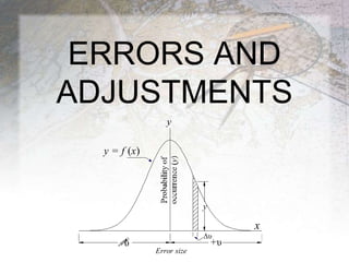
- 1. ERRORS AND ADJUSTMENTS +υυ y = f (x) y Error size x Δυ y
- 2. Example (a) (d)(c)(b) • Which set of shots is more – Accurate? – Precise?
- 3. Precision Example Observation Pacing, p Taping, t EDM, e 1 571 567.17 567.133 2 563 567.08 567.124 3 566 567.12 567.129 4 588 567.38 567.165 5 557 567.01 567.114 • Which observation of a distance is – More precise? – More accurate? e 567.0 567.1 567.2 567.3 567.4 t t t t t eee e Mean of e Mean of t
- 4. Advantages of Least Squares • Errors adjusted according to laws of probability • Easy to perform with today’s computers • Provides a single solution to a set of observations • Forces observations to satisfy geometric closures • Can perform presurvey planning
- 5. Example (cont.) • Construct the 95% confidence interval • From the F0.025 distribution table (D.4) we find – F0.025,24,30 = 2.21 and F0.025,30,24 = 2.14 • Construct the 95% confidence interval 2 1 2 2 2 1 2 2 2.25 1 2.25 2.21 0.49 2.14 0.49 2.14 10.15
- 6. Population versus Sample • Below are random samples having 10 values each. 32.2 30.0 24.2 18.9 17.2 22.4 21.3 21.3 26.4 24.5 28.0 21.2 18.9 33.2 30.2 26.5 25.2 29.0 21.8 26.3 33.9 21.3 21.3 25.2 18.9 19.6 28.5 36.0 27.1 30.6 24.2 24.4 28.5 25.3 32.2 19.6 32.9 21.3 24.0 26.5 μ = 23.84 σ2 = 22.05 μ = 26.03 σ2 = 19.39 μ = 26.24 σ2 = 36.29 μ = 25.89 σ2 = 18.41
- 7. Basics of Error Propagation • Control, distances, directions, and angles all contain random errors • So what are the errors in the computed – Latitudes? – Departures? – Coordinates? – Areas? – And so on? • If we can answer this, we can answer the question, “did our observations meet acceptable closures?”