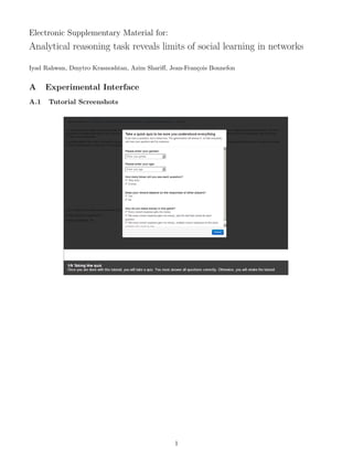
1. Electronic Supplementary Material for:
Analytical reasoning task reveals limits of social learning in networks
Iyad Rahwan, Dmytro Krasnoshtan, Azim Shari↵, Jean-Fran¸ois Bonnefon
c
A
A.1
Experimental Interface
Tutorial Screenshots
1

2. 2

3. 3

4. 4

5. 5

6. A.2
Quiz Questions
Following is the set of quiz questions that participants have to correctly answer before they can proceed to
the experiment. The correct answers are highlighted in bold.
How many times will you see each question?
1. Only once
2. 5 times
Does your reward depends on the responses of other players?
1. Yes
2. No
How do you make money in this game?
1. Every correct response gets me money
2. Not every correct response gets me money, only the last trial counts for each question
3. Not every correct response gets me money, multiple correct responses to the same question only count
as one
6

7. B
Questions
Below is the list of all questions. The first three questions corresponded to the Cognitive Reflection Test
(CRT). These three questions generate an incorrect intuitive answer, which must be inhibited in order to
produce the correct analytic answer [1].
1. [CRT1] In a lake, there is a patch of lily pads. Every day, the patch doubles in size. If it takes 48 days
for the patch to cover the entire lake, how long would it take for the patch to cover half of the lake?
(Answer: 47)
2. [CRT2] If it takes 5 machines 5 minutes to make 5 widgets, how long would it take 100 machines to
make 100 widgets? Write the answer in minutes.
(Answer: 5)
3. [CRT3] A bat and a ball cost $1.10 in total. The bat costs $1.00 more than the ball. How much does
the ball cost?
(Answer: 0.05)
After the three CRT questions, subjects moved on to another series of four questions from the Berlin
Numeracy Test (BNT), which we do not discuss in this article [2]. Being either too easy or too hard, these
questions produced little variance between participants in our networks, and thus did not allow us to test
our hypotheses (see Figure 1 below for a visualization of the responses in the BNT questions). As these
question came after participants had completed the three CRT questions, there is no concern that they could
have contaminated the CRT data that we analyze in this article.
1. [BNT1] Imagine we are throwing a five-sided die 50 times. On average, out of these 50 throws how
many times would this five-sided die show an odd number (1, 3 or 5)?
out of 50 throws.
(Answer: 30)
2. [BNT2] Out of 1,000 people in a small town 500 are members of a choir. Out of these 500 members
in the choir 100 are men. Out of the 500 inhabitants that are not in the choir 300 are men. What is
the probability that a randomly drawn man (not a person) is a member of the choir? (please indicate
the probability in percents)
(Answer: 25)
3. [BNT3] Imagine we are throwing a loaded die (6 sides). The probability that the die shows a 6 is
twice as high as the probability of each of the other numbers. On average, out of these 70 throws, how
many times would the die show the number 6?
out of 70 throws.
(Answer: 20)
4. [BNT4] In a forest 20% of mushrooms are red, 50% brown and 30% white. A red mushroom is
poisonous with a probability of 20%. A mushroom that is not red is poisonous with a probability of
5%. What is the probability that a poisonous mushroom in the forest is red?
(Answer: 50)
7

8. Proportion of correct responses
TOPOLOGY
Full
First Question
Erdos−Renyi
Barabasi−Albert
Second Question
Clustered
Third Question
Baseline
Fourth Qestion
1.00
0.75
0.50
0.25
0.00
1
2
3
4
5
1
2
3
4
5
1
2
3
4
5
1
2
3
4
5
Trial
Figure 1: BNT questions are either too easy or too hard, reducing variance observed in CRT questions.
8

9. C
C.1
Network Structures & Their Properties
The Networks
A network (or graph) consists of a set V vertices (a.k.a. nodes, individuals), and a set E of edges (a.k.a.
connections or links) between them. Elements of E can be denoted by a pair Eij = (i, j) where i, j 2 V .
Each of our experimental sessions ran on one of the four graphs: (1) Barabasi-Albert model; (2) Clustering
graph; (3) Erdos-Renyi model; (4) Full graph. The di↵erent graph structures are visually depicted below.
These graphs were chosen due to significant discrepancy in their measures on the macro (network) and micro
(node) level, as shown below.
Barabasi−Albert model
Clustering graph
Full graph
Erdos−Renyi model
Figure 2: List of graphs
9

10. C.2
Micro Measures
And on the micro level (for each node):
Degree: The degree ki of a vertex i is simply the number of edges incident to this vertex. In a directed
graph, we can distinguish between the out-degree (outgoing edges) and in-degree (incoming edges). In the
present paper, edges are considered undirected.
The di↵erent graph structures we used have significantly varying distributions of node degrees, as shown
below. The degree distribution of the Erdo-Renyi graph follows a Poission distribution, thus most nodes
have a more or less equal number of neighbors (no one is disproportionately popular). In contrasted, in the
Barabasi-Albert graph, the distribution is long-tailed, with a few very highly connected nodes. In the full
graph, everyone has equal degree, since everyone is connected to everyone else. Finally, in the clustering
graph, degrees are more or less identical. However, as we will see below, some nodes are a more privilaged
position in the middle of the graph.
Barabasi model
Erdos−Renyi model
20
20
15
15
10
10
5
5
0
0
5
10
15
0
20
0
Full graph
5
10
15
20
Clustering graph
20
20
15
15
10
10
5
5
0
0
5
10
15
0
20
0
5
10
15
20
Figure 3: Degree distribution
Local clustering coe cient: The local clustering coe cient captures the following intuition: out of all
pairs of friends that i is connected to, how many of those friends are also friends with one another. In other
words:
Ci =
number of triangles connected to node i
number of triples centered around node i
where a triple centred around node i is a set of two edges connected to node i (if the degree of node i is 0
or 1, we which gives us Ci = 0/0, we can set Ci = 0). High local clustering coe cient for node i indicates
that i belongs to a tightly knit group.
More formally, the local clustering coe cient ci is defined as follows:
Ci =
|{Ejk }|
: vj , vk 2 Ni , Ejk 2 E
ki (ki 1)
where ki is the out-degree of vertex i, and Ni = {vj : Eij 2 E} is the set of out-neighbours of vertex i. For
10

11. undirected graphs the value of Ci is normalized as Ci0 = 2Ci . If to rephrase this in the simple words, the
local clustering coe cient of a vertex in a graph shows how close its neighbors are to being a full graph.
The figure below highlights how the distribution of local clustering coe cients varies significantly across
the di↵erent network structures. In particular, nodes in the Erdos-Renyi and Barabasi-Albert graphs have
much lower clustering compared to the Clustering graph. Note that in the full graph, every node has a local
clustering coe cient of 1, since everyone is connected to everyone else.
Betweenness centrality: The betweenness centrality of a node is equal to the number of shortest
paths (among all other vertices) that pass through that node. The higher the number, the more important
is the node, in the sense that there is a small number of hops between that node and the majority of the
network. Mathematically it can be defined as
g(v) =
X
s6=v6=t
st (v)
st
where st is the total number of shortest paths from node s to node t and st (v) is the number of those
paths that pass through v.
The figure below shows that the betweenness centrality of nodes in the Clustering graph vary significantly
(contrast this with the fact that the node degrees in this graph are almost identical to one another).
Clustering coefficient
1
0.5
0
Barabasi model Erdos−Renyi model
Full graph
Clustering graph
Betweenness centrality
60
40
20
0
−20
Barabasi model Erdos−Renyi model
Full graph
Clustering graph
Figure 4: Clustering coe cient, betweenness centrality
C.3
Macro Measures
2|E|
Graph density: In graph theory, graph density is defined as |V |(|V | 1) . Density represents the ratio of
the number of edges to the maximum number of possible edges. Density will therefore have a value in the
interval [0, 1].
Clustering coe cient of a graph: The clustering coe cient of an undirected graph is a measure of the
number of triangles in a graph. The clustering coe cient for the whole graph is the average of the local
clustering coe cients Ci :
n
1X
C=
Ci
n
i=1
11

12. where n is the number of nodes in the network. By definition 0  Ci  1 and 0  C  1.
Diameter: Diameter of the graph is the lenght of the longest shortest path between any two vertices of the
graph.
Macro level parameters for the four classes of networks are summarized in the table below. Note how
the density and diameter of all graphs is almost identical, with the exception of the full graph, which has
maximum density.
graph type
Barabassi
Erdos-Renyi
Full graph
Clustering graph
Density
0.195
0.211
1
0.179
Clustering
0.208
0.158
1
0.714
12
Diameter
4
4
1
5
Number of edges
37
40
190
34

13. D
Evolution of Network States
The figures below show samples of the detailed evolution of correct (blue) and incorrect answers (red) in a
selection of network/question combinations.
Figure 5: Evolution of the game (Barabasi-Albert, question 1)
13

14. Figure 6: Evolution of the game (Barabasi-Albert, question 3)
14

15. Figure 7: Evolution of the game (Full, question 1)
15

16. Figure 8: Evolution of the game (Full, question 2)
16

17. Figure 9: Evolution of the game (Erdos-Renyi, question 1)
17

18. References
[1] Frederick S. Cognitive reflection and decision making.
2005;19(4):25–42.
The Journal of Economic Perspectives.
[2] Cokely ET, Galesic M, Schulz E, Ghazal S, Garcia-Retamero R. Measuring risk literacy: The Berlin
numeracy test. Judgment and Decision Making. 2012;7(1):25–47.
18