1. CIV 2552 – Mét. Num. Prob. de Fluxo e Transporte em Meios Porosos
2013_1
Trab2
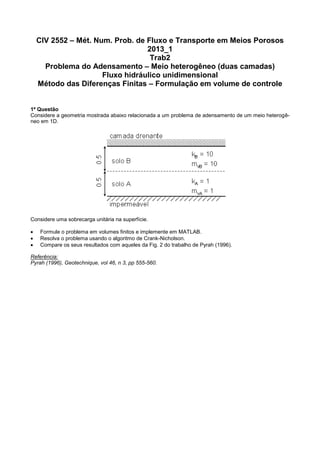
Problema do Adensamento – Meio heterogêneo (duas camadas)
Fluxo hidráulico unidimensional
Método das Diferenças Finitas – Formulação em volume de controle
1ª Questão
Considere a geometria mostrada abaixo relacionada a um problema de adensamento de um meio heterogê-
neo em 1D.
Considere uma sobrecarga unitária na superfície.
Formule o problema em volumes finitos e implemente em MATLAB.
Resolva o problema usando o algoritmo de Crank-Nicholson.
Compare os seus resultados com aqueles da Fig. 2 do trabalho de Pyrah (1996).
Referência:
Pyrah (1996), Geotechnique, vol 46, n 3, pp 555-560.
2. 2ª Questão: Simulação de problema de fluxo em uma camada drenante de areia que liga um rio a
uma escavação
A geometria na figura abaixo mostra o local de uma escavação próxima a um rio. O perfil do solo contém
uma camada areia onde a água deverá passar devido ao rebaixamento de H1 para H2.
A carga q representa a contribuição distribuída da água de chuva na camada de areia.
Dados:
K = 8 x 10
–4
cm/s = 8 x 10
–6
m/s
Ss = 1 x 10
–4
m
–1
q = 1 x 10
–6
m/s
H1 = 40 m
H2 = 5 m
L = 80 m (extensão do domínio 1D)
a = 1 m (largura do modelo 1D)
b = 5 m (espessura da camada de areia)
Condição inicial: h(x) = H1 para t = 0 e x de 0 a L.
Condições de contorno: h(0) = H1 e h(L) = H2.
Determinar h(t) ao longo da camada.
Determinar a vazão de água para dentro da escavação.
Resolva o problema usando o algoritmo implícito de Crank-Nicholson.
3. TECHNICAL NOTE
One-dimensional consolidation of layered soils
I. C. PYRAHÃ
KEYWORDS: consolidation; fabric/structure of soils;
numerical modelling and analysis; pore pressures;
settlement.
INTRODUCTION
The pioneering work of Terzaghi demonstrated
that for a homogeneous clay layer, subjected to an
increase in vertical load under one-dimensional
conditions, the pore water pressure is related to
position within the clay layer z, the time after
application of the load t and the coef®cient of
consolidation cv. While it is widely appreciated
that this is a function of both compressibility mv
and permeability k, it is often assumed that if cv is
constant throughout a layer it is the only parameter
required to predict rates of consolidation even if
the deposit is layered. This apparently reasonable
assumption, however, can lead to some misleading
results and this note, using four simple soil
pro®les, highlights the inadequacies of this ap-
proach for situations where the soil is not
homogeneous.
PROBLEM DEFINITION
The four idealized soil pro®les (Fig. 1) all
consist of two soil layers of equal depth. Only two
soil types (A and B) are considered and for ease of
presentation the coef®cients of compressibility and
permeability for soil A are taken as unity, as is
the unit weight of water ãw. Soil B has values
of compressibility and permeability an order of
magnitude greater than soil A. The coef®cient of
consolidation for both soils is fully de®ned by
these parameters (cv ˆ k/mvãw) and is equal to
one in both cases. The height of each double soil
layer is H, the top is fully drained and the base is
impermeable, i.e. single drainage. The applied load
Pyrah, I. C. (1996). GeÂotechnique 46, No. 3, 555±560
555
Manuscript received 31 March 1995; revised manuscript
accepted 23 August 1995.
Discussion on this technical note closes 2 December
1996; for further details see p. ii.
à Napier University, Edinburgh.
Soil A
Soil B
Soil B
Soil A
Soil B
Soil B
Soil A
Soil A
Free-draining Free-draining
Free-draining Free-draining
Impervious base Impervious base
CASE (i) CASE (ii)
CASE (iii)
Impervious base Impervious base
CASE (iv)
Soil A k = 1
mv = 1
cv = 1
γw = 1Pore fluid
Soil B k = 10
mv = 10
cv = 1
Fig. 1. Assumed soil pro®les
4. p is constant and four con®gurations are consid-
ered
(i) soil A on top of soil B
(ii) soil B on top of soil A
(iii) soil A on top of another layer of soil A
(iv) soil B on top of another layer of soil B.
The last two cases are, of course, not true
layered soils and are simply introduced for com-
parison with the two more interesting soil pro®les.
Soil pro®les (iii) and (iv) represent homogeneous
strata, and Terzaghi's theoretical solution for one-
dimensional consolidation can be applied directly.
Both have the same coef®cient of consolidation
and behave identically in that the variations of
pore water pressure with time and depth will be
the same. The rates of consolidation will also be
identical, although the settlements for case (iv)
will be ten times those for case (iii), as soil B is
ten times more compressible than soil A. Three
methods for predicting settlements for soil pro®les
(i) and (ii) are consolidated below.
PREDICTION PROCEDURES
Approach 1Ðbased on standard average degree of
consolidation curve
If separate oedometer tests were performed on
two soil samples, one taken from soil A and the
other from soil B, each would give the same value
for the coef®cient of consolidation and an engineer
might reasonably consider it appropriate to esti-
mate the time-dependent settlement by using the
standard solution for a homogeneous clay layer for
all four soil pro®les. Using this approach the
predicted pore water pressure isochrones and the
rate of consolidation would be the same for all
cases, irrespective of whether the soil strata are
identical, or whether soil A overlies soil B or vice
versa.
To estimate how the settlement varies with time,
the conventional method is to ®rst estimate the
®nal settlement rF from the compressibility charac-
teristics of the soil and then to multiply this by the
appropriate average degree of consolidation "U to
obtain the settlement rt at a particular time, i.e.
rt ˆ rF
"U (1)
where
rF ˆ
…H
0
pmv dz
"U ˆ
2
1 À
…H
0
ut dz
pH
3
and the pore water pressure ut is a function of z and t
with an initial value equal to the applied pressure p.
For both soil pro®les (i) and (ii) the ®nal
consolidation settlement is a combination of the
settlement due to the compression of soil A (1pH/
2) plus that due to the compression of soil B
(10pH/2), i.e. rF ˆ 5´5 pH. As the average degree
of consolidation, as de®ned above, is independent
of whether soil A or soil B is next to the
permeable boundary, so too is the settlement rt.
Whether this is reasonable is explored below.
Approach 2Ðbased on isochrones from standard
solution
The above solution assumes that the degree of
settlement is the same as the average degree of
consolidation based on the distribution of pore
pressure with depth which, although true for a
uniform deposit, is incorrect for one in which
compressibility varies with depth.
For any clay deposit the pore water pressure in
the soil closest to a free-draining surface will
dissipate much more quickly than that in the soil
furthest away from a free-draining boundary. Thus,
in the early stages of consolidation the surface
settlement will be controlled mainly by the
compressibility of the soil adjacent to the free-
draining boundary, while the compressibility of the
soil away from this boundary will be more
signi®cant during the later stages of consolidation.
In case (i) the more compressible soil (soil B) is
next to the impervious boundary and the settlement
will be much slower than in case (ii), where soil B
overlies the stiffer soil A. The effect of the
different compressibilities must be taken into
account in the solution, and this is not done if
the standard theoretical average degree of con-
solidation/time factor relationship is used.
A more consistent approach is to evaluate the
settlement directly from the change in effective
stress at each point in the soil layer. The change
in effective stress due to the dissipation of the
excess pore pressure is a function of position
and time, and is the difference between the initial
value of the pore pressure p and its current value
ut, i.e.
rt ˆ
…H
0
(p À ut)mv dz (2)
The pore water pressures may be obtained from
the standard isochrones and use of these together
with a different value of mv for each soil layer,
rather than the average degree of consolidation
together with an average value for mv as was done
using approach 1, would seem a more appropriate
procedure. Unfortunately, this approach is still
incorrect for soil pro®les (i) and (ii).
556 PYRAH
5. Correct methodÐbased on mv and k rather than
the single parameter cv
While the settlement prediction using approach
2 takes account of the different compressibilities of
the two soils, no consideration has been given to
the difference in their permeabilities or the effect
this has on the dissipation of pore pressure and the
resulting time-dependent settlements. Correct solu-
tions can be obtained only if solid±¯uid continuity
is taken into account throughout the whole soil
deposit, including layer boundaries. Continuity
between the clay layers requires that the pore
pressures and ¯ow rates in adjacent layers at a
layer interface are the same; this requirement is
ignored in the simple approaches outlined above.
Correct solutions may be obtained using a
variety of analytical and numerical techniques
(Schiffman & Arya, 1977). Numerical techniques
include both ®nite difference and ®nite element
methods based on either a diffusion or a coupled
(Biot) approach. For one-dimensional problems both
give the same solution if formulated correctly,
although care must be taken in calculating
settlements if the diffusion approach is used. If
the isochrones are not interpreted correctly, for
example using equation (1) and an average value
of mv rather than equation (2) with different values
of mv for each soil layer, errors similar to those
discussed in the previous section will be
introduced.
The results reported in this technical note were
obtained using the ®nite element method and a
diffusion approach in which the assemblage mat-
rices are formulated in terms of k and mv rather
than the single parameter cv (Desai, 1979). With
this formulation the nodal pore water pressures are
the only unknowns, and the method is computa-
tionally ef®cient. However, because of possible
errors in the interpretation of the resulting iso-
chrones, the results were checked against solu-
tions obtained using a fully coupled (Biot) ®nite
element program (Abid & Pyrah, 1988). With this
approach, where the unknowns include nodal
displacements as well as pore pressures, the sur-
face settlements are given directly rather than
being dependent on an interpretation of the pore
pressure distributions. Both techniques consider
continuity between connecting elements and, pro-
vided every layer boundary is also an element
boundary, no special considerations are required at
the layer interfaces.
RESULTS
The correct solutions are shown in Figs 2±4 for
all four soil pro®les. As the results are plotted non-
dimensionally (Tv ˆ cv t/H2
), the solutions for soil
pro®les (iii) and (iv) are identical and the same as
the standard Terzaghi solution; these results also
represent the solutions obtained for all four soil
pro®les if approach 1 is used.
Figure 2(a) shows the pore pressure distributions
for soil pro®le (ii) (soil B overlying soil A), Fig.
2(b) shows the standard solution for a uniform soil,
cases (iii) (A/A) and (iv) (B/B), and Fig. 2(c)
shows the isochrones for soil pro®le (i) (A/B). The
solutions for rate of settlement and rate of
dissipation of pore water pressure at the imper-
vious boundary are shown in Figs 3 and 4
respectively. The reasons for the signi®cant differ-
ences in these curves can be understood by
examining the dissipation of excess pore water
pressure (Fig. 2) for each soil pro®le.
For case (i) (Fig. 2(c)), where soil A overlies
soil B, it is the permeability of soil A and the
compressibility of soil B that govern the behaviour.
Because of its high compressibility, soil B has to
express a relatively large amount of water from its
voids during consolidation, but the rate at which
this can be done is mainly controlled by the lower
permeability of the overlying soil. Hence most of
the total settlement, which is due to the compres-
sion of soil B, is correspondingly delayed. Con-
versely, for case (ii) (Fig. 2(a)), where the more
compressible soil lies next to the free-draining top
boundary, most of the settlement occurs relatively
rapidly. As the contribution of soil A to the overall
settlement is small, the rate of settlement is mainly
governed by the consolidation of soil B. As this
soil layer is adjacent to the free-draining boundary
and has a thickness H/2, the rate of settlement is
approximately four times higher than that of the
standard solution. For case (i), where the more
compressible soil is overlain by the less permeable
soil, the rate of settlement is signi®cantly lower;
the results indicate a rate approximately 1/40 of
that for the standard solution.
DISCUSSION
While the correct method for analysing the one-
dimensional behaviour of layered soils has been
known for many years, the examples above
illustrate the signi®cant effect that variations in
permeability and compressibility can have on the
behaviour of a soil deposit. As was intimated by
Wroth (1989), the consolidation of a two-layer soil
may be likened to the heat-conduction problem of
baked Alaska. For those not familiar with this
dessert, it is made by covering ice-cream with
whisked egg white and sugar and placing this in a
very hot oven for a few minutes. The outer
covering bakes quickly to form a crisp shell, while
the ice cream, protected by the low conductivity of
the covering, remains cold. The result is a
delicious sweet, a combination of cold, soft ice
cream surrounded by warm, crisp meringue. This
is analogous to case (i); the analogy for case (ii)
ONE-DIMENSIONAL CONSOLIDATION OF LAYERED SOILS 557
7. would be to surround the whisked egg white with
ice cream and to place this in a very hot oven. It is
unlikely that this has been attempted, but the
outcome would be signi®cantly different from
Baked Alaska and clearly illustrates the difference
between the two cases. (Note: For the analogy to
be strictly correct the values of the thermal
diffusivity k of the meringue and the ice cream
should be identical; k ˆ k/cr where k is thermal
conductivity, c is speci®c heat and r is density.
Although the thermal diffusivity for the two
materials may not be the same, and hence the
analogy with two soils having the same value of cv
not exact, the relative values of thermal conduc-
tivity and of the product of speci®c heat and
density are such that the problem is a useful
illustration of the behaviour of layered materials.)
To return to the examples involving four
Soil profile [B/A]
Uniform soil
Soil profile [A/B]
100
90
80
70
60
50
40
30
20
10
0
1.00E−05 1.00E−04 1.00E−03 1.00E−02 1.00E−01 1.00E+00 1.00E+01 1.00E+02
Elapsed time (TV)Surfacesettlement(%)
Fig. 3. Rate of settlement for different soil pro®les
100
90
80
70
60
50
40
30
20
10
0
1.00E−05 1.00E−04 1.00E−03 1.00E−02 1.00E−01 1.00E+00 1.00E+01 1.00E+02
Elapsed time (Tv)
Excessporewaterpressure(%)
Soil profile [B/A]
Uniform soil
Soil profile [A/B]
Fig. 4. Dissipation of pore water pressure at impervious boundary
ONE-DIMENSIONAL CONSOLIDATION OF LAYERED SOILS 559
8. different soil pro®les: these illustrate the impor-
tance not only of treating a saturated soil as a two-
phase material, including solid±¯uid compatibility
and the effects of time, but also of modelling the
composite nature or fabric of the soil in order to
capture its true behaviour. In geotechnical en-
gineering there are many instances where the
presence of different materials, having different
stress±strain and permeability characteristics, has a
signi®cant effect on the mass behaviour of the soil.
An examination of the effect of the disposition of
such non-uniformities is likely to lead to a better
understanding of soil behaviour. This applies to
both natural and man-made ground.
CONCLUSIONS
Simple examples involving the one-dimensional
consolidation behaviour of layered soils consisting
of two layers with the same value of the coef®cient
of consolidation, but with different compressibility
and permeability characteristics, have been used to
illustrate the importance of adopting correct
procedures in predicting their behaviour. The
examples also illustrate the signi®cant effect that
the arrangement of the different constituents can
have on the behaviour of a soil.
REFERENCES
Abid, M. M. & Pyrah, I. C. (1988). Guidelines for using
the ®nite element method to predict one-dimensional
consolidation behaviour. Comput. Geotech. 5, 213±
226.
Desai, C. S. (1979) Elementary ®nite element method.
Englewood Cliffs, NJ: Prentice-Hall.
Schiffman, R. L. & Arya, S. K. (1977). One-dimensional
consolidation. Numerical methods in geotechnical
engineering (edited by C. S. Desai and J. T.
Christian), pp. 364±398. London: McGraw-Hill.
Wroth, C. P. (1989). Private communication.
560 PYRAH