1. Executive Compensation: Six Questions That Need Answering
by
John M. Abowd and David S. Kaplan
April 1999
Abowd is Professor of Labor Economics at Cornell University, Distinguished
Senior Research Fellow at the United States Bureau of the Census, research
associate of the National Bureau of Economic Research (Cambridge, MA) and
research affiliate of the Centre de Recherche en Economie et Statistique (Paris).
Kaplan is a research economist at the Bureau of Labor Statistics. We are grateful
for financial support from the National Science Foundation (SBER 96-18111). We
also thank Robert Cho and Brian Dunn for providing some of the Towers Perrin
data used in this paper. No confidential data have been used in this paper. Our
data can be accessed at http://old-instruct1.cit.cornell.edu:8000/abowd-john. The
opinions expressed in this paper reflect the views of the authors, and do not
reflect the policies of the Bureau of the Census or the Bureau of Labor Statistics
or the views of other staff members in either organization.
Introduction to Executive Compensation
The big news this year isn’t in the big numbers—it’s in the fine print. Buried in
the latest pay contracts chief executives are signing and the lists of stock-options
they’re salting away in the wall safe are the auguries and portents of things to
come. (Business Week, April 24, 1995, pp. 88.)
As the quotation above suggests, there is a growing realization by the popular business
press that a proper analysis of stock and option holdings is crucial to understanding US executive
compensation practices. The academic economics literature has also come to this conclusion,
although only very recently. Despite being in its infancy, the economics literature on the effects
of stock and options holdings has already yielded large dividends, and has the potential for much
more.

2. In this article, we focus on how this recent advance can be used to address the following
six questions:
1. How much does executive compensation cost the firm?
2. How much is executive compensation worth to the recipient?
3. How well does executive compensation work?
4. What are the effects of executive compensation?
5. How much executive compensation is enough?
6. Could executive compensation be improved?
Murphy (1999) reviews the extensive research on executive compensation. In this article,
we consider, instead, some of the implications of that research and some important directions for
future research. We begin by noting how US CEO compensation policies compare with other
OECD countries. Figure 1 shows an international comparison of the importance of some of the
major components of CEO compensation from 1984-1996, based on data from 12 OECD
countries. Figure 2 shows the analogous comparison for human resource directors. The
components are salary, annual bonus, benefits (including pension), and long-term compensation.
The methodology used to construct the chart is the same as Abowd and Bognanno (1995), and
relies on publicly available data from various governmental statistical agencies, Towers Perrin, a
compensation consulting firm, and other private companies. The estimates shown are for the
domestic national CEO of a company incorporated in the indicated country with $200-500
million in annual sales (1990 dollars).1 Salary is defined as cash compensation that is determined
at the beginning of an annual pay cycle. Annual bonus is defined as cash compensation that is
determined at the end of an annual pay cycle and is based on only one-year’s worth of
performance information. Benefits are the company’s cost to provide retirement income, health
care, and other services, evaluated on an annualized basis. Long-term compensation is the
annualized present value of any cash, or cash-equivalent compensation that is based on outcomes
measured over periods longer than one year.2 The data in this, and subsequent figures, have been
updated for this paper and are available from the authors on request.
1
Our comparative data come from a variety of sources, which target different size companies in the
individual countries. To make the sources comparable, Abowd and Bognanno regression adjusted the compensation
data so that the size of the reference company was 200-500 million 1990 dollars. We note that it is difficult to get
comparative data for native executives (not foreign nationals) when one looks at very large companies because there
are relatively few of them in most OECD countries.
2
Long-term compensation includes stock options (the right to purchase company stock at a given price),
restricted stock (stock that cannot be sold for some specified period of time), performance share plans (formula-
based stock compensation), and cash equivalents of all of the above.
2

3. Not surprisingly, figure 1 shows that US CEOs receive compensation levels that appear
out of line with the other OECD countries, although figure 2 shows that this is not the case for
human resource directors.3 We will see, however, that the high compensation received by US
CEOs is composed of several complex instruments that require a more detailed analysis in order
to understand US compensation systems.
Although figure 1 shows that US CEOs receive higher levels of pay than those in other
OECD countries, comparisons along other dimensions are also useful. Kaplan (1994) compares
Japanese management practices to those in the US. He finds that the sensitivities of cash
compensation and probability of turnover to market returns are not statistically different across
the two countries. One difference is that financial institutions take a more active role in corporate
governance in Japan, particularly following negative earnings. This may explain why turnover
and compensation are more responsive to negative earnings in Japan. Rather than relying on
monitoring from the board of directors, the interests of US CEOs and shareholders are aligned
through higher stock ownership. Overall, however, Kaplan’s conclusion is that the US and
Japanese systems are quite similar.
The Basic Structure of Contingent Executive Compensation
The system has doled out rich rewards—but it can and does impose hefty
penalties on those who don’t perform. More than ever, the boss is likely to lose
his job and his perks when he doesn’t deliver the profits shareholders expect.
(Business Week, April 22, 1996, pp. 102.)
Most of the early economics literature focused on attempts to model the level and
structure of compensation. Unfortunately, data constraints prevented the detailed analyses of
stock and option holdings that have recently proved so useful. The first puzzle for the literature
was explaining why firm size appeared quite important in explaining cross-sectional variability
in compensation, while firm profitability appeared insignificant. Ciscel (1974) noted this fact and
Ciscel and Carroll (1980) hypothesized that the growth of firm size was an important method for
the CEO to increase profitability, so rewards for increasing size might be consistent with
neoclassical theory.
Murphy (1985) made great strides in assessing the incentives provided to executives by
using a panel of firms. He noted that compensation equations estimated on cross-sectional data
look quite different from those that controlled for fixed firm effects. Large firms tend to exhibit
lower rates of return, while paying their executives more than their smaller counterparts. He
showed that firm performance, as measured by the realized shareholder return, is strongly and
positively correlated with managerial remuneration in specifications that controlled for firm
effects. He noted, however, that growth of firm sales is also strongly related to managerial
3
A figure showing that US manufacturing operatives receive compensation levels similar to those in other
OECD countries is available upon request or from the web site mentioned in the acknowledgements. Figures that use
real exchange rates rather than purchasing power parity rates are also available. Real exchange rates are useful to
compare differences in employer costs across countries.
3

4. remuneration. Coughlan and Schmidt (1985) showed that termination decisions are affected by
the firm’s stock market performance, while Deckop (1988) documented that CEO compensation
is positively related to firm profits as a percentage of sales.
Having established the strong statistical link between executive compensation and firm
performance, the literature attempted to assess the magnitude and importance of this link. The
seminal article in this line of inquiry is Jensen and Murphy (1990a), which reported a weak
alignment between shareholder interests and managerial incentives. They estimated that CEO
wealth changes $3.25 for every $1,000 change in shareholder wealth, primarily due to the fact
that the median value for CEO stock holdings as a fraction of shares outstanding was 0.0025 in
1987, the only year for which they collected stock-holdings data from proxy statements. Stock
held by family members and shares held as options exercisable within 60 days were treated
identically to shares owned by the CEO. The remaining $0.75 came from the sum of average pay-
for-performance sensitivities arising from cash compensation, stock-option grants, and threat of
dismissal, which were all estimated with data from the Forbes annual surveys of CEO
compensation. They concluded that CEO compensation policies provided incentives that were
too weak to be consistent with agency theory. Haubrich (1994), however, showed through
calibrations of agency models that such low levels of alignment are reconcilable with agency
theory given reasonable values for CEO risk-aversion parameters. That is, even low levels of
alignment impose significant wealth risk on CEOs, so it is not clear that efficiency would be
enhanced by increasing alignment.
Recently, Hall and Liebman (1998) introduced a great technical innovation in the study of
the sensitivity of executive compensation to changes in shareholder wealth. Using the entire
portfolio of long-term compensation—new awards plus the change in the market value of options
and stock already awarded, they found that CEO wealth changes are significantly larger than
those reported by Jensen and Murphy. They estimate that, in 1994, the mean (respectively,
median) sensitivity of CEO wealth to firm performance is about $25.11 ($5.29) for every $1,000
change in shareholder wealth. Changes in the value of stock-option holdings, which were not
included in the Jensen and Murphy estimate, account for $3.66 ($2.15) of this figure. While Hall
and Liebman note that their estimate of the slope of CEO compensation contracts is quite far
from a benchmark of perfect alignment (which would provide first-best incentives), they do show
through simulations that their estimated level of incentive alignment imposes enormous lifetime
consumption risk on CEOs. This is essentially the same argument Haubrich used to reconcile
agency theory with the data, although Hall and Liebman make this point using a less structural
approach.
As Hall and Liebman demonstrated, examining the annual surveys of executive pay in
Business Week or Forbes cannot provide the information required for analyzing executive
compensation policies. One needs to examine holdings of restricted stock and stock options in
order to address the six questions we consider. Since this is a relatively new innovation for the
literature, we will focus much of our paper on these issues. To begin this analysis we briefly
review option-pricing theory; then, we show the relation between the option pricing hedge ratio
and the slope of the incentive compensation (pay-for-performance) relation.
4

5. Starting with the basics, a typical call option used in a compensation system allows an
executive to purchase a specified number of shares of stock at a fixed exercise price, K.
Typically, options granted to US executives have maturity dates of five to ten years; that is, the
right to purchase the stock at the fixed price expires five to ten years after the grant date. The
option contracts are written to allow the executives the right to exercise before the option
matures (American-style calls). Usually, there are some formal restrictions on early exercise
during the first few years of the option’s life (vesting restrictions). Once the options are fully
vested, less formal mechanisms discourage, but don’t eliminate, early exercise. From the vantage
point of option pricing theory, which we apply below, it is rarely a wealth maximizing strategy to
exercise these options before maturity.
While the Black-Scholes (1973) formula is the most famous tool used for valuing stock
options, the formula is only accurate when the wealth-maximizing exercise strategy is to hold the
options until the expiration date. Since it is well known that the presence of dividends can make
early exercise optimal, we choose to present the binomial pricing formula instead. Unfortunately
this methodology does not yield a closed-form solution, although it can be understood using
simple dynamic programming concepts. We provide an introduction to the binomial option-
pricing model in the mathematical appendix, which we summarize below.
The basic insight of option pricing theory is straightforward. Suppose an investor wants
to replicate the payoff of a call option that is held beyond the current period. As we discuss in
some detail in the appendix, this can be accomplished with a purchase of ∆ shares of stock,
which is partially financed by borrowing B dollars at the riskless interest rate.4 As the stock
price (P) changes over time, the investor need only manage this hedge portfolio by adjusting ∆
and B, without adding funds or taking funds out, to replicate the payoff of the option. Assuming
the option is held beyond the current period, the value of the option at any date must equal the
value of the hedge portfolio at that date because the cash flows for the two assets are identical at
all dates, by construction. Of course, the option may be exercised in the current period, which
yields a payoff of P − K . Combining these two cases yields the following expression for the
value of the option:
C = max[P − K , P∆ − B] .
More importantly for our purposes, ∆ , which is commonly called the hedge ratio, measures the
degree to which the option-holder’s wealth is affected by dollar changes in stock price. The
hedge ratio is the number of shares of the underlying stock held in the hedge portfolio per option.
Hence, the hedge ratio is the derivative of the call value with respect to the price of the
underlying security
∂C ( P, K , T )
= ∆ (P , K , T ) ,
∂P
4
Since the investor borrows money, -B always enters the formulas.
5

6. where T is the time to maturity. See Cox and Rubinstein (1985) for details. We now show that
the key design parameters in the compensation contract from an agency-theoretic point of view,
the expected total compensation and the slope of expected compensation with respect to a change
in the price of the firm’s common stock, can be directly modeled using the riskless hedge call
valuation method.
First we need to establish some notation. We will consider an executive’s compensation
over three periods; let 0 denote the initial period and 1 and 2 denote the subsequent compensation
periods. All subscripts denote the compensation period. We focus on an executive who has been
employed by the firm in periods 0 and 1, and will be employed by the firm in period 2 with
probability π (P2 ) , where P2 denotes the stock price in period 2.
Denote E[V2 (P2 ) P2 ] as the expected value of period 2 compensation, conditional on P2 .
Virtually all of the empirical analyses of executive compensation discussed in this article or in
Murphy (1999) can be interpreted as estimates of
∂ E[V2 (P2 ) P2 ] ∂ E[ln V2 (P2 ) P2 ]
or .
∂P2 ∂ ln P2
We need more notation before proceeding. Denote S t as base salary, Ft as the cost of the benefit
package, and N t as the number of options granted; assume all three depend on Pt . Also denote
S tA as the compensation the executive receives if employed outside the firm and assume that S tA
does not depend on Pt .
Straightforward application of the call valuation arguments we made above, combined with the
results in the appendix, yields the following expression:
 ∂S 2 ∂F2 ∂N 2 
 + + C (P 2 , K 2 , T ) 
 ∂P2 ∂P2 ∂P2
∂ E[V2 (P2 ) P2 ]

= π (P2 ) + N 2 ∆(P2 , K 2 , T ) + N1∆(P2 , K1 , T − 1)
∂P2  
 + N 0 ∆(P2 , K 0 , T − 2 ) 
 
 . (1)
 S 2 + F2 + N 2C (P 2 , K 2 , T ) 
 
∂π (P2 )  + N1 (C (P 2 , K1 , T − 1) − C (P1, K1 , T )) 
+  + N (C (P , K , T − 2 ) − C (P , K , T − 1))
∂P2  0 2 0 1 1

− S A 
 2 
While statistical analysis may be the only method of estimating certain parts of equation
(1), like ∂S 2 ∂P2 , other parts of the equation, like N j , K j , and ∆ are data—parts of the
compensation system design. Unfortunately, most companies do not keep track of these
parameters, even when they use riskless hedge methods to compute the cost of their
6

7. compensation systems. Companies do keep data on certain design features—long-term
compensation eligibility, long-term compensation to salary ratio, grant size, etc.—but these are
only crudely related to the slope of expected total compensation with respect to the stock price.
Thus, the primary challenge in uncovering the true links between pay and performance, and the
reason the Hall and Liebman data set on stock and option holdings is so valuable, is the problem
of estimating the derivative in equation (1) using as much data from the executive’s actual
compensation package as possible.
Core and Guay (1998) address this challenge by introducing an inexpensive algorithm for
estimating the sensitivity of options to stock price ( ∆ ), volatility, and dividend changes using
information available from individual proxies or from the data in Compustat’s Execucomp. The
correlation between their estimate of ∆ and ∆ itself is over 0.99 in their sample, indicating that
their methodology could be a powerful tool for future research.
Note that that restricted stock be can be trivially analyzed in this framework. Restricted
stock can be viewed as an option to purchase stock at an exercise price of zero, which generates a
hedge ratio of one. Since recent empirical work has demonstrated that the vast majority of the
link between shareholder and executive wealth comes from stock and stock-option holdings, we
are now armed with a methodology useful for examining our six questions.
Our discussion below will focus on the role of agency theory, which predicts that stock-
based compensation will align executive and shareholder interests by linking the executive’s
compensation directly to increases in the market value of the company. Less risk-averse
executives require less expected total compensation as the slope of the compensation/stock price
relation increases. Agency theory is really the only viable candidate for a theoretical framework
because it is the only model that predicts that the answer to the first two questions we posed in
the introduction (cost to the company vs. value to the executive) will be different.
Risk aversion plays no role in option-pricing theory since the risk generated by an option
can be eliminated with a hedge portfolio. Agency theory, however, predicts that the employer
must prevent this hedging by the employee; hedging unravels the incentive effects of the option.
A risk-averse employee will therefore value the option below its market price. This wedge
between employer cost and employee value can only be optimal if the firm receives a
productivity benefit from the option grant, since the firm must incur higher costs to retain the
employee.
Question 1: How much does executive compensation cost the firm?
The staggering rise in pay for the good, the bad, and the indifferent has left even
some advocates of pay for performance wondering whether the balance between
the CEO and the shareholder is tilting the wrong way. (Business Week, April 21,
1997, pp. 62)
The analysis of the cost of executive compensation centers on the opportunity cost to the
company of the stock and performance-based components. The cost to the company is the
foregone resources represented by the compensation contract. To estimate the amount of these
7

8. foregone resources we use the riskless hedge argument discussed above: if the executive follows
a wealth maximizing strategy, then the cost of the call option cannot exceed the cost of creating
the hedge portfolio that exactly offsets the cash flows of the executive’s option portfolio. With a
constant dividend yield, the binomial approximation to the riskless hedge provides a reliable
estimate of this cost.
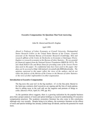
Figure 3 shows estimates of the cost of the 1996 compensation for the CEOs of the S&P
500 companies (Source: Compustat Execucomp, N=496). As can be clearly seen, the values of
the long-term components (options, restricted stock and performance plans) greatly exceed the
other components. These estimates do not include the change in the value of the executive’s
previously awarded stock and stock options. Changes in the value of stock and option holdings
are not relevant in this section since we are considering the cost of creating the hedge portfolio at
the grant date.
There are some conventional problems associated with this method of determining the
cost of executive options. One important problem is that executives exercise the options early
(before the wealth-maximizing date). In this case, the binomial pricing model will lead us to
overstate the cost of the option grants to the firm. To see this, suppose that the firm, anticipating
that it will be forced to pay the executive when he exercises his stock options, decides to create
the hedge portfolio prescribed by the binomial pricing model. This method requires an initial
purchase of company stock and borrowing riskless bonds at the option grant date. Appropriate
management of this fund, adjusting the stock holdings and riskless borrowing at frequent
intervals, will result in the hedge portfolio having the exactly the same value as the executives’
option holdings, assuming optimal exercise behavior. If the executive exercises the option
prematurely, we know that the value of the option and, hence, the value of the hedge portfolio
will both exceed P – K, which is what the executive receives. The firm can therefore liquidate the
hedge portfolio, pay the executive the amount due at early exercise, and have something left
over. Premature exercise therefore reduces the cost of writing the option below that of creating
the hedge portfolio, making the riskless hedge valuation procedure an overestimate of employer
cost.
There are other conventional valuation problems. Interest rate and dividend yield
variation are not priced by the conventional riskless hedge portfolio. Long-term volatility rather
than short-term matters. Finally, the exercise restrictions and vesting of the stock-based
compensation are not reflected in conventional riskless hedge pricing models.
Some of these problems can be addressed. Statistically, we need information on the actual
cash payoffs and exercise dates from a representative sample of executives. If the executives are
exercising earlier than the wealth-maximizing date, then properly constructed hedge portfolios
should accumulate cash, providing an estimate of the difference between actual employer cost
and the cost of the hedge portfolio. If deviations from the constant volatility, dividend yield and
risk-free interest rate assumptions are important, the error in the hedge portfolios should be
significant relative to the cash flows on the options themselves, indicating that more complicated
hedging strategies would be warranted.
8

9. There are also some rather unusual problems in applying option pricing models to
estimate the cost of executive compensation. The binomial pricing model assumes that the
exercise of the option and the creation of the hedge portfolio both have no effect on share price.
Typically, in markets with many small players, this is a reasonable assumption. If one of these
small players, however, is a top executive in the company, the market might anticipate the
incentive effects of his holdings, resulting in a shift of the probability distribution of returns.
An area of compensation research that may grow in importance tries to refine methods for
estimating the cost of executive stock options. A good example of this type of research is Cuny
and Jorion (1995) who note that executive departure typically forces an early exercise of options.
They show that properly accounting for the fact that departure is more likely following poor firm
performance is important for obtaining reliable estimates of option costs. A related study by Saly
(1994) uses a model where stock-option plans are renegotiated after market downturns. Saly’s
empirical results were consistent with the hypothesis that option plans were renegotiated after the
market crash of 1987, i.e., post-crash option grants were significantly larger that pre-crash option
grants.
Question 2: How much is executive compensation worth to the recipient?
The salaries, bonuses, perks and stock gains paid to the top 25 chief executives
over the past five years amount to nearly $1.9 billion. These individuals were
smart and lucky enough to lead highly successful companies during a roaring bull
market. (Forbes, May 20, 1996, pp. 189)
Although the executive can usually realize the wealth maximizing value of the option, his
or her investment portfolio is sub-optimally diversified (the employing company constitutes too
large a proportion of the executive’s wealth portfolio). The executive would, generally, be
willing to exchange the option-based compensation for salary with a present value less than the
current value of the hedge portfolio.
Estimates of this compensating differential are not easy to find. Using as the risk measure
the elasticity of total compensation with respect to the stock price (approximately the share of
stock-based compensation in total compensation) proprietary executive compensation data for
the 1980s show that for every 1% increase in the compensation risk measure, expected total
compensation is 1.8% larger (elasticity of 1.8). The typical compensation package in that era
(20% stock-based compensation for all long-term eligible executives) is, thus about 40% larger,
on average, than total compensation packages with no stock-based compensation. Hall and
Liebman also attempt to estimate this compensating differential and find that it is on the same
order of magnitude for their CEO sample—increases in the executive’s position in the employing
company’s stock or options have a certainty equivalent that is about half of the market value of
the compensation. In the United States, the Financial Accounting Standards Board (FASB) and
the Security and Exchange Commission (SEC), which jointly regulate stock-based compensation
and the form of mandatory disclosures regarding this compensation, should recognize that
executives should disagree over the value of the options in their personal portfolios because they
will have differing attitudes toward risk. The difference between company cost and executive
value is a critical feature of contingent compensation systems. It is one reason why executives
9

10. receive the compensating differentials estimated above. Differences in ability and differences in
bargaining power could also explain these differentials.
We turn now to other differences between employer cost and employee value. Differences
in purchasing power have important effects on the value of pay packages. Interested readers can
request figures identical to figures 1 and 2 except that real exchange rates are used instead of
purchasing power parity rates. The use of purchasing power parity inflates US compensation
relative to compensation in most of the other OECD countries. The reader is reminded that the
data are for significantly smaller companies than were shown in Figure 3.
There are also significant tax and public benefits (pensions) that enter into the executive’s
valuation of the compensation package, especially outside the United States. Figure 4 shows a
comparison of the after-tax, purchasing-power adjusted, compensation of the CEO pay packages
examined in figure 1. All tax payments (income taxes and mandatory employer and employee
public benefit contributions) are shown as negative amounts. Private after-tax compensation is
the dark gray positive amount. The value of public benefits (primarily retirement income and
health care) is shown as the white block at the top. For CEOs, we note that there is considerable
variability in the proportion of the pay package that comes as publicly-provided benefits (France,
Italy and Sweden having the largest components). The tax payments due on the compensation
vary much less than the after-tax compensation itself. Figures analogous to figure 4 for human
resource directors and manufacturing operatives are available upon request.
Question 3: How well does executive compensation work?
You don’t expect a neat correlation in any one year. A chief executive might be
cashing in option gains he had accumulated in other years. But over five years?
Shouldn’t a fat paycheck be matched by shareholder results? (Forbes, May 18,
1998, pp. 232)
As noted earlier, the slope of the compensation/stock price relation is essentially the
option hedge ratio ∆ multiplied by the number of shares held as options. It is impossible to infer
this relation from executive paychecks, which explains the Forbes quote and many others like it.
Hall and Liebman show that, for 1994, the median change in CEO wealth given an increase of
$1,000 in firm value is 5.29. The median elasticity of CEO wealth to firm value is 3.94 in 1994,
which is more than three times the 1980 figure. Perhaps in response to widespread criticism of
CEO pay, the links between CEO wealth and performance have increased dramatically over time.
At the same time as the business press advocated stronger links between pay and performance as
a formula for improved profitability, the connection between stock price and executive wealth
was increasing because of increased stock and stock option holdings. It is difficult to determine
whether these increases in incentive compensation had the predicted effect on stock-market
performance and profitability.
The availability of measures of both compensation and firm performance make executive
compensation a good place to test agency-theoretic models. A simple and direct test of some of
the most basic implications of agency theory is found in Garen (1994). His analysis relies on
Jensen and Murphy’s (1990b) analysis of 430 large firms for which they estimated the sensitivity
10

11. of CEO wealth to changes in shareholder wealth. Garen’s main finding—variables that are
related to greater variability of firm profitability are negatively related to the Jensen and Murphy
estimates of the pay-for-performance sensitivities—is predicted by the theory. More recently,
Aggarwal and Samwick (1999) address these same issues with more complete data. Using
Compustat-Execucomp, which has data on roughly the 1,500 largest publicly-traded US firms,
they also find that pay-for-performance sensitivity is negatively correlated with the variability of
firm stock-market performance, primarily because CEOs of high-variability firms tend to own a
lower percentage of their firm’s stock.
There have been many attempts in the compensation literature to test the relative
performance evaluation (RPE) hypothesis. The basic idea behind RPE is that there are some
identifiable aspects of firm performance that are outside the executive’s control. A market-wide
movement in stock returns is the classic example. A compensation scheme that negatively links
an executive’s wealth to the performance of other firms can therefore reduce the risk necessary to
achieve any level of incentive alignment. Antle and Smith (1986) was the first paper that tested
this hypothesis, but found little evidence that two-digit industry returns affect executive cash
compensation, although they did find some evidence that two-digit industry returns negatively
affect broader definitions of compensation. Barro and Barro (1990) study RPE for CEOs of
banks. They found no evidence that the average stock-market and accounting performance for
other banks within a bank’s region affects the cash compensation of CEOs, though higher
average regional performance makes turnover more likely, as predicted by RPE theory.
Using a broader sample of firms, Gibbons and Murphy (1990) found that the salary plus
bonus of a CEO is increasing in own firm rate-of-return, while decreasing in either industry or
market-wide return, exactly as the theory predicts. They note, however, that industry measures of
rate-of-return have little explanatory power compared to market returns, which seems surprising
since industry returns should more accurately reflect the environment of the firm. They found
similar results for turnover. Janakiraman, Lambert, and Larcker (1992) estimated firm-specific
compensation equations and found results that were, on average, similar to Gibbons and Murphy.
Bertrand and Mullainathan (1999) use annual cash compensation plus the value of stock options
granted to test whether CEOs are rewarded for exogenous shocks in oil prices. They find very
little evidence of RPE and, to the extent that they do find it, it is stronger for negative shocks
than for positive ones.
To our knowledge, the only paper that investigates the RPE hypothesis with data on stock
and option holdings is Aggarwal and Samwick (1999), which finds no evidence of RPE. This is
not surprising, since the instruments that primarily link performance outcomes to executive
wealth, stock and option holdings, have no relative components in them. We therefore conclude
that, despite the obvious attractive features of RPE, it is surprisingly absent from US executive
compensation practices. Why shareholders allow CEOs to ride bull markets to huge increases in
their wealth is an open question.
Gibbons and Murphy (1990), and Aggarwal and Samwick (forthcoming) offer
explanations for the weak evidence in support of RPE. Gibbons and Murphy note that a negative
link between CEO compensation and the performance of rival firms can encourage actions that
lower the performance of rival firms, even at the expense of own-firm performance. Aggarwal
11

12. and Samwick take this argument step further and argue that a positive link between CEO
compensation and rival performance can create incentives that mimic collusive outcomes.
Aggarwal and Samwick also present surprising evidence that, in some industries, CEO
compensation is positively affected by the performance of rival firms. Differences across
industries in the strengths of the links accord well with their theoretical model. Despite the
arguments made in these two papers, we view the weak evidence of RPE as an important puzzle
for executive compensation research.
Question 4: What are the effects of executive compensation?
Despite the soaring pay, many experts argue that the system is working better than
ever. They see the bull market and healthy corporate sector as proof positive that
companies get what they pay for. (Business Week April 21, 1997, pp. 60)
One of the most fundamental questions for the early CEO pay literature was whether or
not incentive contracts actually motivate executives. In particular, the impact of incentives on
stock-market returns has been studied extensively. Before reviewing the literature on the effect of
incentive plans on stock returns, we should stress how difficult it is to obtain guidance on this
subject from economic theory. These difficulties arise for at least two reasons.
The first difficulty is that stock returns have shareholder expectations imbedded in them.
As we mentioned earlier, an option grant might affect the distribution of stock returns for the
company. The forward-looking nature of stock prices might allow this shift to occur prior to the
executive taking any action. In fact, the shift in the distribution of prices, and therefore a current
return reflecting this shift, might occur when shareholders first begin to expect an incentive plan,
which may occur well before the plan is announced and, even more likely, before it is fully
implemented. This could explain why early exercise of options is discouraged, since early (and
unanticipated) exercise could allow executives to reap the benefits of shareholder expectations
without delivering on them.
The second difficulty arises because economic theory does not predict that increases in
incentives necessarily lead to increases in profitability. If firms are providing their executives
with incentives that are close to their profit-maximizing levels, then a small increase in
incentives should lead to almost no change in profitability.
Despite these theoretical difficulties, the effect of incentive plans on stock returns has
been studied extensively. Masson (1971) is the earliest of the studies linking financial incentives
to subsequent performance. He found that firms that provided greater financial incentives for
their CEOs exhibited better stock-market performance over the postwar period, which he
interpreted as evidence that firms systematically provided sub-optimally low incentives. Larcker
(1983) also found a positive stock-market reaction when the adoption of a short-term
compensation plan, a bonus plan based on single-year performance measures, was announced.
Tehranian and Waegelein (1985), however, note that abnormal returns seem to precede the
announcement of the adoption of a short-term compensation plan, making it difficult to interpret
the Larcker result.
12

13. Leonard (1990) found that in his sample of large firms from 1981-85, that companies
with long-term incentive plans exhibited greater increases in return on equity than those without
these plans. Abowd (1990) found that the sensitivity of managerial compensation in one year is
positively related to corporate performance in the next year, although this relationship is much
stronger for market measures of performance than for accounting measures. This result reflects
the difficulty of testing for optimal compensation system design because of the problems,
discussed above, of measuring performance expectations in an efficient capital market and
attempting to estimate a first-order condition for the best design.
When outcomes other than profitability are examined, economic theory can provide clear
guidance. Economic theory certainly predicts that executives will work harder when given larger
incentives to do so. Kahn and Sherer (1990) tested this prediction by examining longitudinal data
from one firm. The firm had two types of incentive programs: bonuses that mainly targeted
higher levels of management, and merit payments available across all managerial levels. They
showed that managers with high sensitivities of bonus payments to subjective performance
evaluations tended to have higher subsequent evaluations, as compared to other managers at that
firm, even after controlling for prior evaluations. They found no significant effects of merit pay
on subsequent performance.
Another important area of research focuses on some unintended effects of incentive plans.
One of the seminal articles in this field is Healy (1985), who studied the effects of non-linear
bonus schemes on managerial accrual and accounting procedures. He found that managers are
more likely to choose income-decreasing accruals (decisions that lower reported profitability)
when their bonus plan’s upper or lower bound is binding, i.e., the pay-for-performance sensitivity
is zero. Note that there is no profit-maximizing rationale for this behavior. It is simply a rational
response by the managers to the incentives they face, even though this behavior might be harmful
to long-term profitability.
Holthausen, Larcker and Sloan (1995) returned to this issue with a data set in which they
can directly identify whether a manager is operating above the upper bound or below the lower
bound of the bonus plan, instead of imputing this as in Healy’s work. They found that managers
do manipulate earnings downward when they are operating above the maximum of their bonus
plan, but they found little evidence that such manipulation occurs when managers are below the
minimum performance level that allows a bonus.
The results on perverse behavior in certain incentive compensation systems lead in an
interesting direction for future research. Healy’s work demonstrates the unfortunate or
unintended effects of incentive plans that contain floors and ceilings. Many case studies also
document unintended effects of high-powered incentives. Is there a downside to increased stock
and option holdings of top executives? Might the increased incentives imposed on today’s
executives be motivating them to do more harm than good? One candidate for an unintended
consequence of high levels of stock and option holdings is that they might encourage excessively
cautious behavior. Since Hall and Liebman showed wealth fluctuations for CEOs can be quite
high, risky but ex-ante profitable projects may seem quite unappealing to executives.
13

14. 6. Question 5: How much executive compensation is enough?
Institutional investors, small shareholders, academics, employees, and even pay
consultants are challenging the vast pay packages given to CEOs. Many of them
express particular dismay that the average CEO paycheck continues to bulge even
in a recession year, when CEOs are demanding sacrifices from their employees
and laying off thousands of workers. The annual largess, many critics say, is out
of step with the times—a hangover of the go-go 1980s that seems egregious in the
frugal 1990s. (Business Week, May 6, 1991, pp. 90)
One of the most common complaints about US CEO compensation policies is how much
CEOs receive relative to others in the firm. Figure 5 shows the after-tax compensation plus
benefits of CEOs as a multiple of the after-tax compensation plus benefits of manufacturing
operatives across 12 OECD counties. This figure shows that US CEOs do, in fact, have
exceptionally high pay relative to manufacturing operatives. Figure 6 shows that this is not true
of US human resource directors.5 The high US CEO relative compensation is particularly striking
when compared to the lower relative pay of German and Japanese CEOs during periods when
they outperformed their US counterparts.
Hallock (1998) provides a small measure of comfort on the issue of “fairness” in the
compensation of CEOs given the welfare of other workers. Contrary to popular opinion, CEOs
do not receive higher compensation when layoffs are announced. Since layoff announcements
have small negative effects on share prices, CEOs are punished for layoffs. This punishment is,
however, quite small and unlikely to be a significant deterrent to layoffs. Dial and Murphy (1995)
use a case study to illustrate that layoffs can be a productivity enhancing strategy, for which the
CEO should be rewarded. That is, while CEOs should not be rewarded directly for layoffs, they
should be rewarded for the increased profitability generated by the layoffs.
The question of “How much is enough?” is an inherently difficult one. We have already
mentioned estimates of the degree to which total compensation rises as compensation risk rises,
but reliable estimates of risk-aversion parameters are necessary to determine if the high
compensation levels in US companies merely reflects a fair risk-return tradeoff. It is difficult to
imagine how these estimates might be obtained.
Kole and Lehn (1996) provide some insight into this issue in their study of airline
deregulation. They found that, relative to CEOs in other industries, CEOs in the airline industry
received increases in their compensation following deregulation, primarily due to increased
stock-option grants. Kole and Lehn provide one example of changes in compensation levels
within US firms in response to environmental changes. Whether observed differences between
compensation levels in the US and other OECD countries reflect optimal responses to
environmental differences or abuses in US compensation systems is a difficult question.
5
Analogs of figures 5 and 6 that use total compensation, which reflects employer costs, are available on
request.
14

15. Question 6: Could executive compensation be improved?
Inside every boardroom, the key issue is how best to link pay to performance. The
standard solution is the stock option, but a number of more rigorous committees
are beginning to wonder if it’s the right answer. The reason harks back to the old
Wall Street saw about not confusing brains with a bull market. Options, by
rewarding CEOs whose stock rises with the tide, may be doing just that. (Business
Week, April 26, 1993, pp. 64)
Since Hall and Liebman demonstrated that CEOs face enormous wealth volatility, firms
should find every possible method to reduce this volatility without reducing incentives. While
this may seem like a daunting task, we mention two possibilities, which we do not claim as our
own insights.
Relative Performance Evaluation. Stock options reward stock price appreciation
regardless of the performance of the economy or sector. Why should CEOs be rewarded for
doing nothing more than riding the wave of a strong bull market? If the exercise price could be
linked to measures like the S&P 500, or an index of close product-market competitors, then
executives would be rewarded for gains in stock price in excess of those explainable by market
factors outside their control. If market-wide stock movements could be netted out of executive
incentive schemes, then equivalent incentives could be provided while reducing the volatility of
the executives’ portfolios.
An interesting research question would be to investigate the extent to which relative
performance evaluation could reduce wealth volatility, while maintaining executive incentives
(hedge ratios multiplied by the number of shares held as options) at their current levels. That is,
how much volatility of executive wealth could be eliminated by not holding them responsible for
share price movements that can be identified as a function of bull or bear markets? These
estimates, combined with estimates of risk-aversion parameters, would lend insight into the value
of resources squandered by a failure to implement relative performance evaluation plans.
Multiple Payoff Criteria. A portfolio of stock options, some with constant exercise prices,
some with exercise prices linked to external criteria (e.g. S&P 500), and some with exercise
prices linked to internal criteria (e.g. division profits or specific executive goals) would provide
more dimensions along which to give direct share price incentives, relative performance
incentives and individual incentives.
While linking executive wealth to stock-market performance has obvious attractive
features, stock-market performance should not be the only measure used. Executives function as
a team and stock-based compensation rewards team performance, but some adjustments should
be made for individual performance to avoid the free rider problem. While the link between the
expected total compensation and the degree of risk in the compensation system is conceptually
well-understood, a better calibration of the compensation sensitivity parameters (slopes or
elasticities) would permit better cost control. In particular, whenever an individual’s contribution
can be isolated, higher-powered incentives can be provided without imposing more
compensation risk on the executive, thus reducing the cost of the compensation.
15

16. Conclusions
We have shown that there are good reasons why the answer to the question “How much
does executive compensation cost the firm?” is different from the answer to the question “How
much is executive compensation worth to the recipient?” for CEO pay. Future executive
compensation research, in the spirit of Hall and Liebman, should be very careful to distinguish
these two concepts. Agency theory remains the only viable candidate for the answer to the
question “How well does executive compensation work?” but the empirical research to date
cannot explain very much about the structure of the optimal contract. For this reason, it is also
hard to answer the questions “What are the effects of executive compensation?” and “How much
executive compensation is enough?” although it is clear that companies can provide both too
little and too much contingent compensation. Finally, we have suggested two fertile areas for
research regarding the question “Could executive compensation be improved?”
One maxim seems clear—whatever happens to CEO pay, the business press will always
have a multitude of kudos and brickbats to hand out every April when they turn their attention to
the recently released proxy statements. Mandatory disclosure of the specifics of American CEO
compensation contracts distinguishes US executives from their colleagues in other countries and
provides the fuel for the empirical study of size and consequences of explicit incentive
compensation programs.
Mathematical Appendix
The binomial pricing methodology assumes that we can divide time into discrete
components, and that the price of the stock can rise or fall in discrete amounts each period. If
dividends were dropped from this exercise, we could derive the Black-Scholes pricing formula,
which is based on a continuous-time model, as a limiting case of the binomial model as the
distance between periods approaches zero.
We follow Cox and Rubinstein (1985) quite closely, and examine a call option to
purchase one share of stock at a fixed exercise price. Suppose that with one period remaining
prior to expiration, the stock price has the following possibilities for the last period.
d (1 − δ ) P or u (1 − δ ) P,
ν ν
where the down and up factors satisfy 0 < d < u , δ is the constant dividend yield, ν = 1 if the
last period is an ex-dividend date and 0 otherwise, and P is the current stock price. When the
expiration date arrives, the option will be worth
Cd = max[0, d (1 − δ ) P − K ] or Cu = max[0, u (1 − δ ) P − K ] ,
ν ν
where K is the exercise price. As Black and Scholes noted when they discussed the riskless
hedge that completed their option pricing model, in the binomial formulation there exist numbers
∆ and B such that holding ∆ shares of stock and borrowing B dollars using riskless bonds is a
payoff-equivalent strategy to holding the option. That is
16

17. dP∆ − rB = C d and uP∆ − rB = C u ,
which implies
Cu − C d dC u − uC d
∆= and B = .
(u − d )P (u − d )r
The payoff from holding the option must be equivalent to the payoff of a portfolio with ∆
shares of stock and B dollars borrowed using riskless bonds. For this reason, this portfolio is
usually called the option hedge portfolio and the dynamic trading strategy associated with the
binomial option pricing formula is called a riskless hedge. If the option is not exercised early,
the value of the option (which we denote C ) must equal the value of this portfolio, namely
P∆ − B . It is possible, however, that the value of exercising the option prior to the last period
( P − K ) exceeds P∆ − B , in which case the option is exercised early.
The value of the option is, therefore,
C = max[P − K , P∆ − B] .
More importantly for our purposes, ∆ , which is commonly called the hedge ratio, measures the
degree to which the option-holder’s wealth is affected by dollar changes in stock price. The
hedge ratio is the number of shares of the underlying stock held in the hedge portfolio per option.
While the analysis thus far has focused on the period prior to expiration, we can apply dynamic
programming techniques to derive the call option value for 2, 3, …, N periods prior to expiration.
As the interval associated with a period tends toward zero, we can express the value of the call
option as C (P, K , T ) , where T is the amount of time until the option expires. Regardless of time
to maturity, the hedge ratio can be expressed as a function of u , d , the current stock price, and
the possible values for the option in the following trading period as shown above. Hence, the
hedge ratio is the derivative of the call value with respect to the price of the underlying security
∂C ( P, K , T )
= ∆ (P , K , T )
∂P
Consider an executive currently employed at a given firm. Let period 0 denote the
executive’s initial compensation period. Let P0 denote the value of the employing firm’s stock at
the end of period 0. The executive receives total compensation with a cost to the company given
by
S0 + F0 + N 0C ( P0 , K 0 , T )
where S0 is salary, F0 is the periodic cost of the benefit package, N 0 is the number of call
options awarded, K 0 is the exercise price of these call options and T is the time to expiration of
the call options. At the end of period 1, a new stock price P is realized. The executive remains
1
employed at this firm with probability π ( P ) . If separated the executive receives alternative
1
17

18. compensation S1A , which does not depend upon P. At the end of period 1, the executive receives
a new stock option grant of N1 shares at exercise price K1 expiring in T years. Salary and
benefits costing S1 + F1 are also paid at this time. A comparable exercise occurs at the beginning
of period 2.
We now consider the realized and expected future compensation of a mid-career
executive, which we will interpret as the values in the model above at the end of period 1. The
executive’s realized compensation at the end of period 1, assuming continued employment, is
V1 = S1 + F1 + N1C ( P , K1 , T1 ) + N 0 (C ( P , K 0 , T − 1) − C ( P0 , K 0 , T ) ) ,
1 1
where the first three terms are comparable to compensation awarded in the initial period and the
final term represents the capital gain or loss on the stock options awarded in the first period.
Viewed as a function of P2 , the executive’s expected future compensation at the end of period 2
is
 S 2 + F2 + N 2C (P2 , K 2 , T ) 
 
E[V2 (P2 ) P2 ] = π (P2 ) + N1 (C (P2 , K1 , T − 1) − C (P , K1 , T ))
1  + (1 − π (P2 ))S 2 .
A
 + N (C (P , K , T − 2) − C (P , K , T − 1))
 0 2 0 1 0 
References
Abowd, John M. “Does Performance-based Compensation Affect Corporate Performance?”
Industrial and Labor Relations Review, 43(3), February 1990, pp. 52S-73S.
Abowd, John M. and Bognanno, Michael. “International Differences in Executive and
Managerial Compensation,” in R. B. Freeman and L. F. Katz, eds. Differences and
Changes in Wage Structures (Chicago: University of Chicago Press for the NBER, 1995),
pp. 67-103.
Aggarwal, Rajesh and Samwick, Andrew A. “The Other Side of the Tradeoff: The Impact of
Risk on Executive Compensation.” Journal of Political Economy, 107(1), February 1999,
pp. 65-105.
Aggarwal, Rajesh and Samwick, Andrew A. “Executive Compensation, Strategic Competition,
and Relative Performance Evaluation: Theory and Evidence,” Journal of Finance,
forthcoming.
Antle, Rick and Smith, Abbie “An Empirical Investigation of the Relative Performance
Evaluation of Corporate Executives.” Journal of Accounting Research, 24(1), Spring
1986, pp. 1-39.
Barro, Jason and Barro, Robert J. “Pay, Performance, and Turnover of Bank CEOs.” Journal of
Labor Economics, 8(4), October 1990, pp. 448-81.
18

19. Bertrand, Marianne and Sendhil Mullainathan, “Are CEOs Rewarded for Luck? A Test of
Performance Filtering,” Princeton University working paper, 1999.
Black, Fisher and Scholes, Myron, “The Pricing of Options and Corporate Liabilities,” Journal of
Political Economy, 81(3), 1973, pp. 637-59.
Byrne, John A. “How High Can CEO Pay Go?” Business Week, April 22, 1996, pp. 100-106.
Byrne, John A. “Executive Pay: The Party Ain’t Over Yet” Business Week, May 6, 1993, pp. 56-
64.
Byrne, John A. “The Flap Over Executive Pay?” Business Week, May 6, 1991, pp. 90-96.
Byrne, John A. and Lori Bongiorno “CEO Pay: Ready For Takeoff.” Business Week, April 24,
1995, pp. 88-94.
Ciscel, David H. “Determinants of Executive Compensation.” Southern Economic Journal,
40(4), April 1974, pp. 613-17.
Ciscel, David H. and Carroll, Thomas M. “The Determinants of Executive Salaries: An
Econometric Survey.” Review of Economics and Statistics, 62(1), February 1980, pp. 7-
13.
Core, John and Guay, Wayne. “Estimating the Incentive Effects of Executive Stock Option
Portfolios.’’ Mimeo, The Wharton School, University of Pennsylvania, November 1998.
Coughlan, Anne T. and Schmidt, Ronald M. “Executive Compensation, Management Turnover,
and Firm Performance: An Empirical Investigation.” Journal of Accounting and
Economics, 16(1-2-3), January-April-July 1993, pp. 43-66.
Cox, John C. and Rubinstein, Mark. Options Markets. New Jersey: Prentice-Hall, Inc., 1985.
Cuny, Charles J. and Jorion, Philippe. “Valuing Executive Stock Options with Endogenous
Departure.” Journal of Accounting and Economics, 20(2), September 1995, pp. 193-205.
Deckop, John R. “Determinants of Chief Executive Officer Compensation.” Industrial and
Labor Relations Review, 41(2), January 1988, pp. 215-26.
Dial, Jay and Murphy, Kevin J. “Incentives, Downsizing, and Value Creation at General
Dynamics.” Journal of Financial Economics, 37(3), March 1995, pp. 261-314.
“Did They Earn It?” Forbes, May 18, 1998, pp. 232.
Garen, John E. “Executive Compensation and Principal-Agent Theory.” Journal of Political
Economy, 102(6), December 1994, pp. 1175-99.
Gibbons, Robert and Murphy, Kevin J. “Relative Performance Evaluation for Chief Executive
Officers.” Industrial and Labor Relations Review, 43(3), February 1990, pp. 30S-51S.
19

20. Hall, Brian J. and Liebman, Jeffrey B. “Are CEOs Really Paid Like Bureaucrats.” Quarterly
Journal of Economics, 111(3), August 1998, pp. 653-91.
Hallock, Kevin F. “Layoffs, Top Executive Pay, and Firm Performance.” American Economic
Review, 88(4) September 1998, pp. 711-23.
Hardy, Eric S. “America’s Highest Paid Bosses.” Forbes, May 20, 1996, pp. 184-89.
Healy, Paul M. “The Effect of Bonus Schemes on Accounting Decisions.” Journal of Accounting
and Economics, 7(1-3), September 1985, pp. 85-107.
Holthausen, Robert W., Larcker, David F, and Sloan, Richard G. “Annual Bonus Schemes and
the Manipulation of Earnings.” Journal of Accounting and Economics, 19(1), February
1995, pp. 29-74.
Janakiraman, Surya N., Lambert, Richard A., and Larcker, David F. “An Empirical Investigation
of the Relative Performance Evaluation Hypothesis.” Journal of Accounting Research,
30(1), Spring 1992, pp. 53-69.
Jensen, Michael C. and Murphy, Kevin J. “Performance Pay and Top-Management Incentives.”
Journal of Political Economy, 98(2), April 1990, pp. 225-64 (a).
Jensen, Michael C. and Murphy, Kevin J. “It’s Not How Much You Pay, but How.” Harvard
Business Review, 68(3), May-June 1990, pp. 138-53 (b).
Kahn, Lawrence M. and Sherer, Peter D. “Contingent Pay and Managerial Performance.”
Industrial and Labor Relations Review, 43(3), February 1990, pp. 107S-20S.
Kaplan, Steven N. “Top Executive Rewards and Firm Performance: A Comparison of Japan and
the United States.” Journal of Political Economy, 102(3), June 1994, pp. 510-46.
Kole, Stacey and Lehn, Kenneth “Deregulation and the Adaptation of Governance Structure: The
Case of the U.S. Airline Industry.’’ Mimeo, Simon Graduate School of Business
Administration, University of Rochester, July 1996.
Larcker, David F. “The Association Between Performance Plan Adoption and Corporate Capital
Investment.” Journal of Accounting and Economics, 5(1), 1983, pp. 3-30.
Leonard, Jonathan S. “Executive Pay and Firm Performance.” Industrial and Labor Relations
Review, 43(3) February 1990, pp. 13S-29S.
Masson, Robert T. “Executive Motivations, Earnings, and Consequent Equity Performance.”
Journal of Political Economy, 79(6), 1971, pp. 1278-92.
Murphy, Kevin J. “Corporate Performance and Managerial Remuneration: An Empirical
Analysis.” Journal of Accounting and Economics, 7(1-3), April 1985, pp. 11-42.
20

21. Murphy, Kevin J. “Executive Compensation,” in Orley Ashenfelter and David Card, eds.,
Handbook of Labor Economics, Volume 3, 1999, forthcoming.
Reingold, Jennifer. “Executive Pay.” Business Week, April 21, 1997, pp. 58-66.
Saly, P. Jane “Repricing Stock Options in a Down Market.” Journal of Accounting and
Economics, 18(3), November 1994, pp. 325-56.
Tehranian, Hassan and Waegelein, James F. “Market Reaction to Short-Term Executive
Compensation Plan Adoption.” Journal of Accounting and Economics, 7(1-3), April
1985, pp. 131-44.
21

23. 1996
1992
1988
United States 1984
1996
1992
1988
Total Compensation of CEOs at Purchasing Power Parity Exchange Rates
United Kingdom 1984
1996
1992
1988
Switzerland 1984
Long term compensation
1996
1992
1988
Sweden 1984
1996
1992
(12 OECD Countries 1984-1996)
1988
Spain 1984
1996
All benefits and perquisites
1992
Country - Year
1988
Netherlands 1984
1996
Figure 1
1992
23
1988
Japan 1984
1996
1992
1988
Base + bonus
Italy 1984
1996
1992
1988
Germany 1984
1996
1992
1988
France 1984
1996
1992
1988
Canada 1984
1996
1992
1988
1000 Belgium 1984
800
600
400
200
0
rates
Thousands of 1998 US dollars at annual average OECD ppp

24. 1996
1992
United States 1984
1996
1992
Total Compensation of HRDs at Purchasing Power Parity Exchange Rates
United Kingdom 1984
1996
1992
Switzerland 1984
Long term compensation
1996
1992
Sweden 1984
1996
1992
(12 OECD Countries 1984-1996)
Spain 1984
1996
All benefits and perquisites
Country - Year
1992
Netherlands 1984
Figure 2
1996
24
1992
Japan 1984
1996
1992
Base + bonus
Italy 1984
1996
1992
Germany 1984
1996
1992
France 1984
1996
1992
Canada 1984
1996
1992
Belgium 1984
250
200
150
100
50
0
rates
Thousands of 1998 US dollars at annual average OECD ppp

25. 1996 CEO Compensation S&P 500
(thousands of 1998 US Dollars)
Salary + Annual bonus
Benefits
2,043
Performance-based long
2,887
term
Restricted stock
149
381 Options
399
Figure 3
25

26. 1996
1992
1988
United States 1984
1996
1992
1988
Total Taxes, Private After Tax Compensation, and Public Benefits for CEOs
United Kingdom 1984
1996
1992
1988
Public benefits
Switzerland 1984
1996
1992
1988
Sweden 1984
1996
1992 Private net compensation
(12 OECD Countries 1984-1996)
1988
Spain 1984
1996
1992
Country - Year
1988
Netherlands 1984
1996
Figure 4
1992
26
1988
All payroll and income taxes
Japan 1984
1996
1992
1988
Italy 1984
1996
1992
1988
Germany 1984
1996
1992
1988
France 1984
1996
1992
1988
Canada 1984
1996
1992
1988
Belgium 1984
-200
-400
800
600
400
200
0
rates
Thousands of 1998 US dollars at annual average OECD ppp

27. 1996
1992
1988
United States 1984
1996
1992
Ratio of CEO After-Tax Compensation and Benefits To That Of Manufacturing
1988
United Kingdom 1984
1996
1992
1988
Switzerland 1984
1996
1992
1988
Sweden 1984
1996
1992
1988
Spain 1984
Operatives (1984-1996)
1996
1992
Country - Year
1988
Netherlands 1984
Figure 5
1996
27
1992
1988
Japan 1984
1996
1992
1988
Italy 1984
1996
1992
1988
Germany 1984
1996
1992
1988
France 1984
1996
1992
1988
Canada 1984
1996
1992
1988
Belgium 1984
25
20
15
10
5
0
Ratio to Manufacturing Operative