Suicide is the third leading cause of death for adolescents .docx

Suicide is the third leading cause of death for
adolescents and young people in the United
States. The etiology of suicide in this popula-
tion has eluded policy makers, researchers,
and communities. Although many suicide pre-
vention programs have been developed and
implemented, few are evidence-based in their
effectiveness in decreasing suicide rates. In one
northern California community, adolescent sui-
cide has risen above the state’s average. Two
nurses led an effort to develop and implement
an innovative grassroots community suicide
prevention project targeted at eliminating any
further teen suicide. The project consisted of
a Teen Resource Card, a community resource
brochure targeted at teens, and education for
the public and school officials to raise awareness
about this issue. This article describes this proj-
ect for other communities to use as a model.
Risk and protective factors are described, and a
comprehensive background of adolescent sui-
cide is provided.
AbstrAct
A Community Takes Action
Linda M. Pirruccello, MsN, rN
Earn
4.0 Contact Hours

34 Copyright © SLACK Incorporated
I
t is not uncommon for ado-
lescents to think about end-
ing their lives (Gould &
Kramer, 2001; Rueter, Holm,
McGeorge, & Conger, 2008),
although thinking about suicide
does not always lead to suicide
attempts (Pelkonen & Mart-
tunen, 2003). The national
2007 Youth Risk Behavior Sur-
vey of a representative sample
of students in grades 9 through
12 indicated 14.5% of students
seriously considered attempting
suicide, 11.3% made a suicide
plan, and 6.9% attempted suicide
during the 12 months preceding
the survey (Eaton et al., 2008). It
is for this reason that the nation’s
public health agenda objectives
for Healthy People 2010 prioritized
adolescent suicide prevention ef-
forts (U.S. Department of Health
and Human Services, 2000).
Youth often experience tre-
mendous stress, confusion, and
hopelessness related to situa-

tions in their lives, schools, and
communities, which too often
lead young people to consider
suicide as their only solution.
Despite alarmingly high youth
suicide rates, there has been
limited research on how to com-
prehensively predict, treat, and
prevent suicide among youth
(Macgowan, 2004). Indeed, the
complexities of youth suicide
behavior continue to confound
policy makers, professionals,
communities, and researchers.
Although public attention and
awareness of youth suicide has
increased during the past 2 de-
cades in the United States, sui-
cide was still the third leading
cause of death in 2006 among
youth ages 15 to 24, accounting
for 4,189 deaths (Centers for
Disease Control and Preven-
tion [CDC], 2009a).
One purpose of this article
is to raise awareness of the
problem of adolescent suicide,
which is the first step in the
development of suicide preven-
tion strategies. Another pur-
pose is to encourage and inspire
nurses and other health care
professionals to become agents
of change and leaders within
their communities in prevent-

ing youth suicide. This article
describes one suicide preven-
tion project that led to the
implementation of a grassroots
community-based intervention
program targeting youth. This
project provides an example of
nurses leading and collaborat-
ing within their local commu-
nity in an effort to eliminate
adolescent suicide.
scoPe of the ProbLeM
Suicide is rare in childhood
and early adolescence but in-
creases every year as children
age (Pelkonen & Marttunen,
2003). Suicide rates in the
United States for male adoles-
cents between ages 15 and 19 are
four times higher than the rates
for their female peers (CDC,
2009b). Due to the growing risk
of suicide with increasing age,
there is a critical need to tar-
get suicide prevention efforts in
adolescents (Pelkonen & Mart-
tunen, 2003) and develop sui-
cide prevention programs.
During the past several de-
cades, adolescent (ages 15 to
19) suicide rates in the United
States have shifted. In 1950, sui-

cide rates for both sexes for ages
15 to 19 were 2.7 per 100,000.
By 1990, these rates reached a
peak rate of 11.1 per 100,000.
Subsequently, from 1990 to
2003, the rates significantly de-
clined in this age group from
11.1 to 7.3 per 100,000 (Na-
tional Center for Health Sta-
tistics, 2005). According to a
recent CDC report, adolescent
suicide rates for 2003-2004 dem-
onstrated the largest increase
in annual suicide rates during
the past 15 years, from 11.61
to 12.65 per 100,000 (CDC,
2007b). The problem may actu-
ally be worse than these figures
indicate because suicide rates
may be underreported and mis-
classified (Institute of Medicine
[IOM], 2002). These trends
A Community Takes Action
Linda M. Pirruccello, MsN, rN
©
2
01
0/
iS
to
ck

ph
ot
o.
co
m
/D
aw
n
H
ud
so
n/
O
lg
a
Ax
yu
tin
a
35Journal of Psychosocial nursing • Vol. 48, no. 5, 2010
demonstrate the urgency to pri-
oritize suicide prevention efforts
for adolescents.

Explanations for the differing
rate trends are not easily under-
stood. Some researchers assert
the increased youth suicide rates
of the 1990s were attributed to
greater exposure of this popula-
tion, particularly boys, to drugs
and alcohol (Gould, Green-
berg, Velting, & Shaffer, 2003).
The possible reasons for declin-
ing adolescent suicide rates be-
tween 1990 and 2003 in the
United States include the use
of antidepressant medication in
treating depressed adolescents
(Olfson, Shaffer, Marcus, &
Greenberg, 2003), the reduction
of alcohol use (Birckmayer &
Hemenway, 1999), and more re-
strictive gun control laws (Web-
ster, Vernick, Zeoli, & Mangan-
ello, 2004).
risk ANd Protective
fActors
During the past two decades,
there has been increased under-
standing about factors contribut-
ing to suicide, although the etiol-
ogy of youth suicide has not been
determined (Evans et al., 2005).
Primary risk factors and protec-
tive factors (those that mitigate
against youth suicide) have been

suggested (IOM, 2002). How-
ever, the manner in which pro-
tective and risk factors influence
suicide remains unclear (Lubell
& Vetter, 2006).
risk factors
Risk factors reported to con-
tribute to suicidal behavior in-
clude the following:
l Presence of psychiatric
illness, with depression being
most common (Burns & Patton,
2000).
l Previous history of sui-
cide attempts (Hawton, Zahl, &
Weatherall, 2003).
l Low family and peer sup-
port (Kerr, Preuss, & King,
2005).
l Physical and sexual abuse
(Bensley, Van Eenwyk, Spieker,
& Schoder, 1999).
l Victimization (Borowsky,
Ireland, & Resnick, 2001).
l Same-sex orientation (Rus-
sell & Joyner, 2001).

l Serotonin deficiency (Ka-
mali, Oquendo, & Mann, 2001).
l Having a family mem-
ber who had attempted suicide
(Brent & Mann, 2006).
l Access to firearms (Miller,
Azrael, Hepburn, Hemenway, &
Lippmann, 2006).
The relationship of substance
abuse to adolescent suicide is
unclear (Rowan, 2001). Certain
psychosocial factors or stressors
are also suggested to interact and
contribute to increased youth sui-
cide risk. These stressors include
family discord, poor parent-child
relationships, family history of
suicide behavior, problems in
school, breakup of a close rela-
tionship, arguments and fights, a
friend attempting or completing
suicide, and relocation (Mac-
gowan, 2004).
Protective factors
Protective factors in general
are consistent with psychologi-
cal health, but their influence
in providing protection against
youth suicide remains uncertain
(Evans et al., 2005). Leading

protective factors include having
the following (World Health Or-
ganization, 2000):
l Supportive family and
adult relationships.
l Connectedness to school
and other organizations.
l Good social and coping
skills.
l Self-confidence in one’s
own abilities.
l Willingness to seek help
with difficulties.
Additional protective factors
include access to evaluation and
ongoing mental health resources,
community support, and con-
flict resolution and skill building
(CDC, 2007a).
suicide PreveNtioN
APProAches
Although multiple risk and
protective factors have been
identified with suicide behavior
in adolescence, further research
is needed concerning the impact
they have on current interven-
tion strategies. Many different

approaches have been taken
to prevent suicide behavior in
youth; however, few programs
have been empirically tested for
their effectiveness (Evans et al.,
2005). Given the range of sug-
gested risk and protective factors
influencing youth suicide behav-
ior, prevention efforts focusing
on reducing risk factors and pro-
moting protective factors should
tAbLe 1
AdoLesceNt suicide PreveNtioN Project strAtegies
Community-Wide
Consciousness Raising
Suicide Prevention Education for Parents,
Students, Educators, and Counselors
• Designing and distributing a
teen resource card
• Design and distribute the Teen Resource Card
for local adolescents
• Developing program
resources
• Development and dissemination of a local
crisis intervention resource brochure targeted to
adolescents
• Measuring outcomes • Goal: to eliminate adolescent suicides

incorporate and integrate the ex-
pertise of both health and non-
health related sectors including
the school system, community,
government, business, religion,
human services, and health or-
ganizations (Davidson, Ross, &
Silverman, 2001).
coMMuNity suicide
PreveNtioN Project
One local community in ru-
ral northern California that had
adolescent suicide rates higher
than the state average recognized
the seriousness of the problem
of youth suicide and decided to
take action to address the prob-
lem. The project’s suicide pre-
vention strategies captured the
entire community’s energy and
attention, and formalized a col-
laborative partnership between
individuals and agencies from
both health and non-health
community sectors.
The program, led by nurses,
included senior and junior high
school educators, youth leaders,

school counselors, civic leaders,
mental health professionals, po-
lice officers, probation officers,
religious leaders, local hospital
officials, concerned parents, high
school students, and media. The
objectives of this project were to
develop new suicide prevention
strategies and to augment exist-
ing programs. The suicide pre-
vention project focused primarily
on raising community awareness
about youth suicide and provid-
ing local adolescents with easy
access to local community crisis
intervention resources. The proj-
ect strategies focused on three
areas (Table 1).
Project goals
The four goals of the adolescent
suicide prevention project were:
l Elimination of adolescent
suicide as measured by a zero
adolescent suicide rate on the
annual coroner’s report.
l Improved community
agency collaboration.
l Increased community
awareness about identifying at-
risk and high-risk youth.

l Enhanced awareness about
accessible crisis response and
referral sources.
Project Planning
The project began when a
small group of concerned citi-
zens gathered to discuss the
problem. Community stake-
holders understood that the
problem required a multidisci-
plinary collaborative approach
and would involve the entire
community, including schools,
social services, faith-based or-
ganizations, law enforcement,
town council, health care orga-
nizations, youth services, local
media, teens, and concerned
community members.
Organizers contacted leaders
from these groups by telephone
inviting them to join in the ef-
fort to identify possible interven-
tions to eliminate local teen sui-
cide. More than 30 community
members came together, finding
common ground. Initially, the
community group met bimonthly
during a 6-month period to final-
ize and adopt project interven-
tions. The primary considerations
in the initial 6 months included

identifying innovative solutions
to the problem; recruiting local
teens to lead and make project
decisions; developing a budget
and identifying existing funding
resources; identifying timelines
and the project completion date;
identifying all agency and com-
munity stakeholders; and identi-
fying barriers and solutions to the
project implementation.
Project Prevention
strategies
The three project prevention
strategies included developing a
wallet-size card; creating a local
resource brochure; and providing
suicide prevention education for
parents, students, and counselors
(Table 1). The teen card and re-
source brochure were developed
and designed by local teens; both
were distributed 6 months after
the planning phase.
Teen Resource Card. The main
prevention strategy was a plastic
credit card style and wallet-size
Teen Resource Card (Figure).
Teens were invited to develop
and design their card to maximize
buy-in. They worked together
with community stakeholders to
formulate goals. The goals the

tAbLe 2
AdoLesceNt suicide PreveNtioN Project budget
Program Element Budget
Suicide prevention education for parents, students, educators,
and counselors (lecturer fee and meeting room rental)
$1,200
Design and development of resource guide, a tri-fold color
brochure printed on quality paper ($1.20 per brochure)
$1,900
Design and distribution of Teen Resource Card ($1.50 per card,
plus graphic designer fee and distribution costs)
$3,000
Conduct research to measure effectiveness of Teen Resource
Card (statistician consulting fees to assist in survey instrument
development and analysis of collected data, paper and printing
costs, and student incentives)
$1,100
Total $7,200
teens chose included immediate
access to help, simplicity of use,

and 24-hour crisis telephone
numbers. The principle of com-
munity connectedness, includ-
ing a spiritual component and
guaranteed confidentiality, in-
formed the process, and it was
decided the card design would
display peer support. Participat-
ing businesses requested that for
discounts to be displayed on the
back of the card, an expiration
date for these offers should also
be printed.
The card included both the
key resource telephone numbers
as well as discounts at local eat-
eries and businesses frequented
by youth. The card had to offer
immediate access to crisis re-
sources. The final version of the
card displayed three main 24-
hour crisis telephone numbers.
The crisis telephone numbers
were services offering support
for substance abuse, mental
health issues, homelessness and
runaways, sexual assault crisis
intervention, and unplanned
pregnancy help. The card was
designed to be simple to use,
small enough to carry in a wal-
let, and attractive to encourage
teens to carry it.

A total of 2,000 Teen Re-
source Cards were distributed
within the community dur-
ing a 2-year period. The total
number of cards produced was
determined by the total popula-
tion of the local high schools,
which was 1,600 students. Ad-
ditional cards were ordered for
distribution in local restaurants
and coffee shops, physician of-
fices, movie theaters, hospital
emergency department wait-
ing areas, and all teen gather-
ing places community wide.
The original 2,000 cards were
ordered at an estimated cost of
$1.50 per card (Table 2). The
cards were made available at no
cost to the youth. Student lead-
ers in each age group were pro-
vided cards to share with their
peers. Three hundred cards
were estimated to be needed
each academic year for incom-
ing 9th-grade students.
Local Resource Brochure. The
second resource was a tri-fold
brochure that included infor-
mation on a wide range of ser-
vices. The contact telephone
numbers included more than
100 local resources and nation-
al 24-hour crisis hot-line tele-
phone numbers that provide

physical and mental health ser-
vices, social services, substance
abuse treatment, sexual assault
and physical abuse help, home-
less shelters, employment and
transportation services, and
leisure activities. All telephone
resources provided were verified
by the nurse leaders.
Community-Wide Educa-
tion. The third project preven-
tion strategy was to provide
community-wide education to
raise awareness about the risk
and protective factors for sui-
cide. The education included
information on evidence-based
prevention strategies and refer-
ral resources in the community
to increase the response and re-
ferral of suicidal youth.
A mental health profes-
sional with expertise in youth
suicide behavior was sought to
focus on the topics. A large va-
riety of community venues that
could accommodate a diverse
community audience including
high school students, interested
community members, school
counselors, teachers, and other
professionals was investigated.
Venues could range from do-

nated space in schools and
churches to rented spaces in a
large meeting hall. Speakers
were sought and asked to do-
nate their services or were pro-
vided an honorarium. A larger
estimated fee was also proposed
to attract a nationally known
mental health expert in adoles-
cent and youth suicide.
Project budget
The budget to implement the
project was $7,200 (Table 2).
Among the financial contribu-
tors were a local hospital, com-
munity service organizations,
local businesses, private donors,
and churches; grant funding
was also provided by the local
high school. Eleven hundred
dollars of the budget were allot-
ted for statistician consultation
fees in survey instrument devel-
opment, analysis of collected
data, and student incentives to
participate in the survey.
PiLot survey
One year after the initial dis-
tribution of the Teen Resource
Card, a pilot survey was con-
ducted with local high school
students (grades 9 through 12).

The survey was developed by
the nurse leaders and consisted
Figure. Teen resource card. A third panel (not
pictured) featured discount offers from local
businesses.
of 17 items that were scored us-
ing a 4-point Likert scale. The
survey sought to determine
teens’ opinions on the follow-
ing three domains of the card:
awareness of the card, motiva-
tion to use the card, and useful-
ness of the card.
Students were asked to rate
items such as “I am carrying the
teen card every day,” “I find the
teen card easy to use,” and “I
like to carry the teen card be-
cause of the telephone numbers
available.” Survey items were
positively worded. Two open-
ended questions were added at
the end of the survey instru-
ment to provide teens an op-
portunity to comment about
the design of the card or sug-
gest any changes they thought
could be useful. Demographic
information collected included

gender and grade level. Due to
the preliminary nature of this
project, survey reliability and
validity were not evaluated.
The pilot survey was admin-
istered to two groups of high
school students by a univer-
sity nursing student supervised
by the nurse leaders. The first
group consisted of students in
grades 9 and 10 (n = 22), and
the second group consisted of
students in grades 11 and 12
(n = 18). Permission to admin-
ister the survey was granted by
the teacher of record for the
class. The purpose of the pilot
survey was described to the stu-
dents, and students were assured
that taking the survey was vol-
untary and that their responses
would be anonymous.
Composite variables for each
of the three areas of interest were
calculated by summing survey
items in each of the three do-
mains to identify level of aware-
ness of the card, motivation, and
perceived usefulness of the card.
The higher the score, the stron-
ger the positive evaluation for
the three areas of interest.

Student responses from the
two open-ended questions were
examined. Forty-one percent of
students did not respond to the
two questions. Of those students
who commented, results sug-
gested older students (ages 15 to
18) were aware of the card and
found the card useful and easy to
use, although they did not always
carry it. In addition, the older
students were motivated to use
the card because of the resource
telephone numbers and not only
just because of the design or dis-
counts. In contrast, the majority
of younger students (ages 13 to
14) were unaware of the card and
did not know the kind of infor-
mation on the card. However, a
smaller percentage of younger
students indicated they were mo-
tivated to carry and use the card
because of the resource numbers.
Older students’ suggestions
about the card design included
changing the color scheme to
black and white. One of the
older students suggested the
design on the card should be
more “artistic” to make people
feel more at ease about calling
the telephone numbers on the
card, whereas another older stu-

tAbLe 3
resuLts of the PiLot study oN the teeN resource cArd
Question Ages Response
What, if anything, about the Teen
Resource Card especially pleased you?
13 to 14 • “How it helps when we need it.”
• “That it can be there for help, if you need it or if you are
going through a lot of problems.”
15 to 18 • “I think that it is good to give the kids resources.”
• “I feel that the card would be helpful to kids who are
struggling.”
• “The discounts are good.”
• “I like it ’cause it gives you numbers that you can call if
you need someone to talk to.”
What, if anything, would you change on
the design or information on the Teen
Resource Card?
13 to 14 • “Design’s good ’cause the information is easy to
find.”
15 to 18 • “Different colors but black and white.”
• “I would make the design more artistic—to make people
feel more safe calling.”

dent suggested leaving the card
design alone because it “looked
cool.” Only one younger stu-
dent commented about the card
design, stating the “Design’s
good ’cause the information is
easy to find.” Examples of stu-
dent responses are shown in
Table 3.
PreLiMiNAry outcoMes
Prior to implementation of
this project, the local commu-
nity was rocked four times by
unrelated deaths of four male
adolescents—two from drug
overdose and two from suicide.
One year after the card distri-
bution, an adolescent suicide
rate of zero was recorded on the
local coroner’s report. It is im-
possible, however, to determine
whether this reduction was a
direct consequence of the cards.
Data related to unsuccessful sui-
cide attempts are not available.
This is a pilot study to ex-
plore and understand how the
cards could provide an effec-
tive intervention to eliminate
successful suicide attempts in

adolescents. Due to the pre-
liminary nature of this project,
no scientific outcome data are
available.
coNcLusioN
Teenage suicide is a national
health crisis. Nurses, by virtue
of the nature of their role as
health care professionals, are
ideally positioned in the com-
munity to provide leadership in
the development of programs
designed to prevent suicide.
The suicide adolescent preven-
tion project demonstrates how
nurses in one community took
a leadership role in the design
and implementation of a sui-
cide prevention project. The
model they developed could be
duplicated and used by nurses
in other communities.
refereNces
Bensley, L.S., Van Eenwyk, J.V., Spieker,
S.J., & Schoder, J. (1999). Self-
reported abuse history and adoles-
cent problem behaviors. I. Antiso-
cial and suicidal behaviors. Journal of
Adolescent Health, 24, 163-172.
Birckmayer, J., & Hemenway, D. (1999).

Minimum-age drinking laws and
youth suicide, 1970-1990. American
Journal of Public Health, 89, 1365-
1368.
Borowsky, I.W., Ireland, M., & Resnick,
M.D. (2001). Adolescent suicide at-
tempts: Risks and protectors. Pediat-
rics, 107, 485-493.
Brent, D.A., & Mann, J.J. (2006). Fa-
milial pathways to suicidal behav-
ior—Understanding and preventing
suicide among adolescents. New
England Journal of Medicine, 355,
2719-2721.
Burns, J.M., & Patton, G.C. (2000). Pre-
ventive interventions for youth sui-
cide: A risk factor-based approach.
Australian and New Zealand Journal of
Psychiatry, 34, 388-407.
Centers for Disease Control and Preven-
tion. (2007a). Suicide prevention. Sci-
entific information: Risk and protective
factors. Retrieved from http://www.
cdc.gov/ncipc/dvp/Suicide/suicide_
risk_pfactors.htm
tion. (2007b). Suicide trends among
youths and young adults aged 10-24
years—United States, 1990-2004.
Morbidity and Mortality Weekly Re-
port, 56, 905-908.

tion. (2009a). Ten leading causes of
death and injury (charts). Retrieved
from http://www.cdc.gov/injury/
wisqars/LeadingCauses.html
tion. (2009b). WISQARS injury mor-
tality reports, 1999-2006. Retrieved
from http://webappa.cdc.gov/sasweb/
ncipc/mortrate10_sy.html
Davidson, L., Ross, V., & Silverman,
M.M. (2001). Background papers
to the National Suicide Prevention
Conference: An overview and per-
spective. Suicide and Life-Threatening
Behavior, 31(Suppl. 1), 1-5.
Eaton, D.K., Kann, L., Kinchen, S.,
Shanklin, S., Ross, J., Hawkins, J.,
et al. (2008). Youth risk behavior
surveillance—United States, 2007.
Morbidity and Mortality Weekly Report
Surveillance Summaries, 57(SS4), 1-
131.
Evans, D.L., Foa, E.B., Gur, R.E., Hen-
din, H., O’Brien, C.P., Seligman,
M.E.P., et al. (Eds.). (2005). Treat-
ing and preventing adolescent men-
tal health disorders: What we know
and what we don’t know. A research
agenda for improving the mental health
of our youth. New York: Oxford Uni-

versity Press.
Gould, M.S., Greenberg, T., Velting,
D.M., & Shaffer, D. (2003). Youth
suicide risk and preventive interven-
tions: A review of the past 10 years.
Journal of the American Academy of
Child and Adolescent Psychiatry, 42,
386-405.
Gould, M.S., & Kramer, R.A. (2001).
Youth suicide prevention. Suicide and
Life-Threatening Behavior, 31(Suppl.
1), 6-31.
Hawton, K., Zahl, D., & Weatherall, R.
(2003). Suicide following deliberate
self-harm: Long-term follow-up of
patients who presented to a general
hospital. The British Journal of Psy-
chiatry, 182, 537-542.
Institute of Medicine. (2002). Reducing
suicide: A national imperative. Re-
trieved from National Academies
Press website: http://www.nap.edu/
openbook.php?isbn=0309083214
1. Nurses can provide focused and innovative interventions to
address critical
concerns of youth suicide in a community.
2. Youth suicide is still the third-leading cause of death in ages
12 to 19 and
increases every year as children age, indicating the need for
new suicide

prevention strategies.
3. Adolescents can be motivated and supported to become
agents of change
among their peers.
Do you agree with this article? Disagree? Have a comment or
questions?
Send an e-mail to the Journal, at [email protected]
We’re waiting to hear from you!
k e y P o i N t s
Kamali, M., Oquendo M.A., & Mann,
J.J. (2001). Understanding the neu-
robiology of suicidal behavior. De-
pression and Anxiety, 14, 164-176.
Kerr, C.R., Preuss, L.J., & King, C.A.
(2005). Suicidal adolescents’ so-
cial support from family and peers:
Gender-specific associations with
psychopathology. Journal of Abnor-
mal Child Psychology, 34, 103-114.
Lubell, K.M., & Vetter, J.B. (2006).
Suicide and youth violence preven-
tion: The promise of an integrated
approach. Aggression and Violent Be-
havior, 11, 167-175.
Macgowan, M.J. (2004). Psychosocial

treatment of youth suicide: A system-
atic review of the research. Research
on Social Work Practice, 14, 147-162.
Miller, M., Azrael, D., Hepburn, L.,
Hemenway, D., & Lippmann, S.J.
(2006). The association between
changes in household firearm own-
ership and rates of suicide in the
United States, 1981-2002. Injury
Prevention, 12, 178-182.
National Center for Health Statistics.
(2005). Health, United States, 2005
with chartbook on trends in the health of
Americans. Retrieved from http://www.
cdc.gov/nchs/data/hus/hus05.pdf
Olfson, M., Shaffer, D., Marcus, S.C., &
Greenberg, T. (2003). Relationship
between antidepressant medication
treatment and suicide in adoles-
cents. Archives of General Psychiatry,
60, 978-982.
Pelkonen, M., & Marttunen, M. (2003).
Child and adolescent suicide: Epide-
miology, risk factors, and approaches
to prevention. Paediatric Drugs, 5,
243-265.
Rowan, A.B. (2001). Adolescent sub-
stance abuse and suicide. Depression
and Anxiety, 14, 186-191.
Rueter, M.A., Holm, K.E., McGeorge,

C.R., & Conger, R.D. (2008). Ado-
lescent suicidal ideation subgroups
and their association with suicidal
plans and attempts in young adult-
hood. Suicide and Life-Threatening
Behavior, 38, 564-575.
Russell, S.T., & Joyner, K. (2001). Ado-
lescent sexual orientation and suicide
risk: Evidence from a national study.
American Journal of Public Health, 91,
1276-1281.
U.S. Department of Health and Hu-
man Services. (2000). Healthy people
2010 online documents. Retrieved
from http://www.healthypeople.gov/
Document/
Webster, D.W., Vernick, J.S., Zeoli,
A.M., & Manganello, J.A. (2004).
Association between youth-focused
firearm laws and youth suicides. Jour-
nal of the American Medical Associa-
tion, 292, 594-601.
World Health Organization. (2000). Pre-
venting suicide: A resource for teachers
and other school staff. Retrieved from
http://www.who.int/mental_health/
media/en/62.pdf
Ms. Pirruccello is Assistant Professor
of Nursing, California State University,
Chico, Chico, California.

The author discloses that she has
no significant financial interests in any
product or class of products discussed
directly or indirectly in this activity,
including research support.
Address correspondence to Linda
M. Pirruccello, MSN, RN, Assistant
Professor, California State University,
Chico, 400 West First Street, Chico,
CA 95929-0200; e-mail: [email protected]
yahoo.com.
Submitted: July 17, 2009
Accepted: January 26, 2010
Posted: March 22, 2010
doi:10.3928/02793695-20100303-01
Copyright of Journal of Psychosocial Nursing & Mental Health
Services is the property of SLACK
Incorporated and its content may not be copied or emailed to
multiple sites or posted to a listserv without the
copyright holder's express written permission. However, users
may print, download, or email articles for
individual use.

273
Monopoly
Monopoly: one parrot.
9
273
A firm that creates a new drug may receive a patent that gives it
the right to be the monopoly
or sole producer of the drug for up to 20 years. As a result, the
firm can charge a price much
greater than its marginal cost of production. For example, one
of the world’s best-selling drugs,
the heart medication Plavix, sold for about $7 per pill but can
be produced for about 3¢ per pill.
Prices for drugs used to treat rare diseases are often very high.
Drugs used for certain rare
types of anemia cost patients about $5,000 per year. As high as
this price is, it pales in com-
parison with the price of over $400,000
per year for Soliris, a drug used to treat a
rare blood disorder.1
Recently, firms have increased their
prices substantially for specialty drugs in
response to perceived changes in will-
ingness to pay by consumers and their
insurance companies. In 2008, the price
of a crucial antiseizure drug, H.P. Acthar
Gel, which is used to treat children
with a rare and severe form of epilepsy,
increased from $1,600 to $23,000 per

vial. Two courses of Acthar treatment
for a severely ill 3-year-old girl, Reegan
Schwartz, cost her father’s health plan
about $226,000. Steve Cartt, an execu-
tive vice president at the drug’s manu-
facturer, Questcor, explained that this
price increase was based on a review
of the prices of other specialty drugs
and estimates of how much of the price
insurers and employers would be willing
to bear.
In 2013, 107 U.S. drug patents expired, including major
products such as Cymbalta and
OxyContin. When a patent for a highly profitable drug expires,
many firms enter the market
1When asked to defend such prices, executives of
pharmaceutical companies emphasize the high
costs of drug development—in the hundreds of millions of
dollars—that must be recouped from a
relatively small number of patients with a given rare condition.
Brand-Name and
Generic Drugs
Managerial
Problem
274 CHAPTER 9 Monopoly
W hy can a firm with a patent-based monopoly charge a high
price? Why might a brand-name pharmaceutical’s price rise
after its patent expires? To answer these questions, we need to

understand the decision-making
process for a monopoly: the sole supplier of a good that has no
close substitute.3
Monopolies have been common since ancient times. In the fifth
century b.c., the
Greek philosopher Thales gained control of most of the olive
presses during a year
of exceptionally productive harvests. The ancient Egyptian
pharaohs controlled the
sale of food. In England, until Parliament limited the practice in
1624, kings granted
monopoly rights called royal charters to court favorites.
Particularly valuable royal
charters went to companies that controlled trade with North
America, the Hudson
Bay Company, and with India, the British East India Company.
In modern times, government actions continue to play an
important role in creating
monopolies. For example, governments grant patents that allow
the inventor of a new
product to be the sole supplier of that product for up to 20
years. Similarly, until 1999,
the U.S. government gave one company the right to be the sole
registrar of Internet
domain names. Many public utilities are government-owned or
government-protected
monopolies.4
3Analogously, a monopsony is the only buyer of a good in a
given market.
4Whether the law views a firm as a monopoly depends on how
broadly the market is defined. Is the
market limited to a particular drug or the pharmaceutical
industry as a whole? The manufacturer of

the drug is a monopoly in the former case, but just one of many
firms in the latter case. Thus, defining
a market is critical in legal cases. A market definition depends
on whether other products are good
substitutes for those in that market.
and sell generic (equivalent) versions of the brand-name drug.2
Generics account for nearly
70% of all U.S. prescriptions and half of Canadian
prescriptions.
Congress, when it passed laws permitting generic drugs to
quickly enter a market after a
patent expires, expected that patent expiration would
subsequently lead to sharp declines in
drug prices. If consumers view the generic product and the
brand-name product as perfect
substitutes, both goods will sell for the same price, and entry by
many firms will drive the price
down to the competitive level. Even if consumers view the
goods as imperfect substitutes,
one might expect the price of the brand-name drug to fall.
However, the prices of many brand-name drugs have increased
after their patents expired
and generics entered the market. The generic drugs are
relatively inexpensive, but the brand-
name drugs often continue to enjoy a significant market share
and sell for high prices. Even
after the patent for what was then the world’s largest selling
drug, Lipitor, expired in 2011,
it continued to sell for high prices despite competition from
generics selling at much lower
prices. Indeed, Regan (2008), who studied the effects of generic
entry on post-patent price
competition for 18 prescription drugs, found an average 2%

increase in brand-name prices.
Studies based on older data have found up to a 7% average
increase. Why do some brand-
name prices rise after the entry of generic drugs?
2Under the 1984 Hatch-Waxman Act, the U.S. government
allows a firm to sell a generic product after
a brand-name drug’s patent expires if the generic-drug firm can
prove that its product delivers the
same amount of active ingredient or drug to the body in the
same way as the brand-name product.
Sometimes the same firm manufactures both a brand-name drug
and an identical generic drug, so
the two have identical ingredients. Generics produced by other
firms usually differ in appearance
and name from the original product and may have different
nonactive ingredients but the same
active ingredients.
2759.1 Monopoly Profit Maximization
Unlike a competitive firm, which is a price taker (Chapter 8), a
monopoly can
set its price. A monopoly’s output is the market output, and the
demand curve a
monopoly faces is the market demand curve. Because the market
demand curve
is downward sloping, the monopoly (unlike a competitive firm)
doesn’t lose all its
sales if it raises its price. As a consequence, a profit-
maximizing monopoly sets its
price above marginal cost, the price that would prevail in a
competitive market.
Consumers buy less at this relatively high monopoly price than

they would at the
competitive price.
In this chapter,
we examine six
main topics
Main Topics 1. Monopoly Profit Maximization: Like all firms, a
monopoly maximizes profit by
setting its output so that its marginal revenue equals marginal
cost.
2. Market Power: A monopoly sets its price above the
competitive level, which
equals the marginal cost.
3. Market Failure Due to Monopoly Pricing: By setting its price
above marginal cost,
a monopoly creates a deadweight loss because the market fails
to maximize total
surplus.
4. Causes of Monopoly: Two important causes of monopoly are
cost factors and
government actions that restrict entry, such as patents.
5. Advertising: A monopoly advertises to shift its demand curve
so as to increase its
profit.
6. Networks, Dynamics, and Behavioral Economics: If its
current sales affect a
monopoly’s future demand curve, a monopoly may charge a low
initial price so
as to maximize its long-run profit.

All firms, including competitive firms and monopolies,
maximize their profits by
setting quantity such that marginal revenue equals marginal cost
(Chapter 7). Chapter 6
demonstrates how to derive a marginal cost curve. We now
derive the monopoly’s
marginal revenue curve and then use the marginal revenue and
marginal cost curves
to examine how the manager of a monopoly sets quantity to
maximize profit.
Marginal Revenue
A firm’s marginal revenue curve depends on its demand curve.
We will show that
a monopoly’s marginal revenue curve lies below its demand
curve at any positive
quantity because its demand curve is downward sloping.
Marginal Revenue and Price. A firm’s demand curve shows the
price, p,
it receives for selling a given quantity, q. The price is the
average revenue the firm
receives, so a firm’s revenue is R = pq.
A firm’s marginal revenue, MR, is the change in its revenue
from selling one more
unit. A firm that earns ΔR more revenue when it sells Δq extra
units of output has
a marginal revenue of
MR =
ΔR
Δq
.

If the firm sells exactly one more unit (Δq = 1), then its
marginal revenue, MR, is
ΔR (= ΔR/1).
The marginal revenue of a monopoly differs from that of a
competitive firm
because the monopoly faces a downward-sloping demand curve,
unlike the com-
petitive firm. The competitive firm in panel a of Figure 9.1
faces a horizontal
demand curve at the market price, p1. Because its demand curve
is horizontal,
the competitive firm can sell another unit of output without
reducing its price.
As a result, the marginal revenue it receives from selling the
last unit of output
is the market price.
Initially, the competitive firm sells q units of output at the
market price of p1, so
its revenue, R1, is area A, which is a rectangle that is p1 * q. If
the firm sells one more
unit, its revenue is R2 = A + B, where area B is p1 * 1 = p1.
The competitive firm’s
marginal revenue equals the market price:
ΔR = R2 - R1 = (A + B) - A = B = p1.
A monopoly faces a downward-sloping market demand curve, as
in panel b of
Figure 9.1. (So far we have used q to represent the output of a

single firm and Q to
represent the combined market output of all firms in a market.
Because a monopoly
FIGURE 9.1 Average and Marginal Revenue
p,
$
p
er
u
ni
t
q q + 1 q, Units per year
p1
(a) Competitive Firm
Demand curve
A B
Q Q + 1 Q, Units per year
p1
p2
p,
$

p
er
u
ni
t
(b) Monopoly
Demand curve
A B
C
Revenue with One
More Unit,
R2
Initial Revenue,
R1
Marginal Revenue,
R2 - R1
Competition A A + B B = p1
Monopoly A + C A + B B − C = p2 − C
The demand curve shows the average revenue or price
per unit of output sold. (a) The competitive firm’s mar-
ginal revenue, area B, equals the market price, p1. (b) The
monopoly’s marginal revenue is less than the price p2 by
area C, the revenue lost due to a lower price on the Q

units originally sold.
is the only firm in the market, q and Q are identical, so we use
Q to describe both the
firm’s output and market output.
The monopoly, which initially sells Q units at p1, can sell one
extra unit only
if it lowers its price to p2 on all units. The monopoly’s initial
revenue, p1 * Q, is
R1 = A + C. When it sells the extra unit, its revenue, p2 * (Q +
1), is R2 = A + B.
Thus, its marginal revenue is
ΔR = R2 - R1 = (A + B) - (A + C) = B - C.
The monopoly sells the extra unit of output at the new price, p2
, so its extra rev-
enue is B = p2 * 1 = p2. The monopoly loses the difference
between the new price
and the original price, Δp = (p2 - p1), on the Q units it
originally sold: C = Δp * Q.
Therefore the monopoly’s marginal revenue, B - C = p2 - C, is
less than the price
it charges by an amount equal to area C.
Because the competitive firm in panel a can sell as many units
as it wants at the
market price, it does not have to cut its price to sell an extra
unit, so it does not
have to give up revenue such as Area C in panel b. It is the
downward slope of the

monopoly’s demand curve that causes its marginal revenue to be
less than its price.
For a monopoly to sell one more unit in a given period it must
lower the price on all
the units it sells that period, so its marginal revenue is less than
the price obtained
for the extra unit. The marginal revenue is this new price minus
the loss in revenue
arising from charging a lower price for all other units sold.
The Marginal Revenue Curve. Thus, the monopoly’s marginal
revenue curve
lies below a downward-sloping demand curve at every positive
quantity. The relation-
ship between the marginal revenue and demand curves depends
on the shape of
the demand curve.
For linear demand curves, the marginal revenue curve is a
straight line that starts
at the same point on the vertical (price) axis as the demand
curve but has twice the
slope. Therefore, the marginal revenue curve hits the horizontal
(quantity) axis at
half the quantity at which the demand curve hits the quantity
axis. In Figure 9.2, the
demand curve has a slope of -1 and hits the horizontal axis at 24
units, while the
marginal revenue curve has a slope of -2 and hits the horizontal
axis at 12 units.
We now derive an equation for the monopoly’s marginal
revenue curve. For a
monopoly to increase its output by one unit, the monopoly
lowers its price per unit
by an amount indicated by the demand curve, as panel b of

Figure 9.1 illustrates.
Specifically, output demanded rises by one unit if price falls by
the slope of the
demand curve, Δp/ΔQ. By lowering its price, the monopoly
loses (Δp/ΔQ) * Q
on the units it originally sold at the higher price (area C), but it
earns an additional p
on the extra output it now sells (area B). Thus, the monopoly’s
marginal revenue is
MR = p +
Δp
ΔQ
Q. (9.1)
Because the slope of the monopoly’s demand curve, Δp/ΔQ, is
negative, the last
term in Equation 9.1, (Δp/ΔQ)Q, is negative. Equation 9.1
confirms that the price is
greater than the marginal revenue, which equals p plus a
negative term and must
therefore be less than the price.
We now use Equation 9.1 to derive the marginal revenue curve
when the monop-
oly faces the linear inverse demand function (Chapter 3)
p = 24 - Q, (9.2)
that Figure 9.2 illustrates. Equation 9.2 shows that the price
consumers are willing to

pay falls $1 if quantity increases by one unit. More generally, if
quantity increases by
ΔQ, price falls by Δp = -ΔQ. Thus, the slope of the demand
curve is Δp/ΔQ = -1.
We obtain the marginal revenue function for this monopoly by
substituting into
Equation 9.1 the actual slope of the demand function, Δp/ΔQ = -
1, and replacing
p with 24 - Q (using Equation 9.2):
MR = p +
Δp
ΔQ
Q = (24 - Q) + (-1)Q = 24 - 2Q. (9.3)
Figure 9.2 shows a plot of Equation 9.3. The slope of this
marginal revenue curve
is ΔMR/ΔQ = -2, so the marginal revenue curve is twice as
steep as the demand
curve.
Using Calculus Using calculus, if a firm’s revenue function is
R(Q), then its marginal revenue function is defined as
MR(Q) =
dR(Q)
dQ
.
For our example, where the inverse demand function is p = 24 -
Q, the revenue
function is

R(Q) = (24 - Q)Q = 24Q - Q2. (9.4)
Deriving a
Monopoly’s
Marginal Revenue
Function
p,
$
p
er
u
ni
t
Demand
(p = 24 – Q )
Perfectly elastic, ε→ –∞
Perfectly
inelastic, ε = 0
Elastic, ε < –1
Inelastic, –1 < ε < 0
ε = –1
Δp = –1
ΔQ = 1ΔQ = 1

ΔMR = –2
Q, Units per day
24
12
0 12 24
Marginal Revenue
(MR = 24 – 2Q )
FIGURE 9.2 Elasticity of Demand and Total, Average, and
Marginal Revenue
The demand curve (or average revenue curve),
p = 24 - Q, lies above the marginal revenue curve,
MR = 24 - 2Q. Where the marginal revenue equals
zero, Q = 12, the elasticity of demand is ε = -1. For
larger quantities, the marginal revenue is negative, so the
MR curve is below the horizontal axis.
Marginal Revenue and Price Elasticity of Demand. The marginal
revenue at any given quantity depends on the demand curve’s
height (the price)
and shape. The shape of the demand curve at a particular
quantity is described by
the price elasticity of demand (Chapter 3), ε = (ΔQ/Q)/(Δp/p) 6
0, which tells
us the percentage by which quantity demanded falls as the price

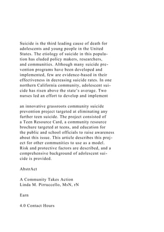
increases by 1%.
At a given quantity, the marginal revenue equals the price times
a term involving
the elasticity of demand (Chapter 3):5
MR = p¢1 + 1
ε
≤. (9.5)
5By multiplying the last term in Equation 9.1 by p/p (=1) and
using algebra, we can rewrite the
expression as
MR = p + p
Δp
ΔQ
Q
p
= pJ1 + 1
(ΔQ/Δp)(p/Q)
R .
The last term in this expression is 1/ε, because ε =
(ΔQ/Δp)(p/Q).
Q&A 9.1
Given a general linear inverse demand curve p(Q) = a - bQ,
where a and b are posi-
tive constants, use calculus to show that the marginal revenue
curve is twice as steeply
sloped as the inverse demand curve.

Answer
1. Differentiate a general inverse linear demand curve with
respect to Q to determine its
slope. The derivative of the linear inverse demand function with
respect to Q is
dp(Q)
dQ
=
d(a - bQ)
dQ
= -b.
2. Differentiate the monopoly’s revenue function with respect to
Q to obtain the mar-
ginal revenue function, then differentiate the marginal revenue
function with
respect to Q to determine its slope. The monopoly’s revenue
function is R(Q) =
p(Q)Q = (a - bQ)Q = aQ - bQ2. Differentiating the revenue
function with
respect to quantity, we find that the marginal revenue function
is linear,
MR(Q) = dR(Q)/dQ = a - 2bQ.
Thus, the slope of the marginal revenue curve,
dMR(Q)
dQ
= -2b,

is twice that of the inverse demand curve, dp/dQ = -b.
Comment: Note that the vertical axis intercept is a for both the
inverse
demand and MR curves. Thus, if the demand curve is linear, its
marginal
revenue curve is twice as steep and intercepts the horizontal
axis at half the
quantity as does the demand curve.
By differentiating Equation 9.4 with respect to Q, we obtain the
marginal
revenue function, MR(Q) = dR(Q)/dQ = 24 - 2Q, which is the
same as
Equation 9.3.
According to Equation 9.5, marginal revenue is closer to price
as demand becomes
more elastic. Where the demand curve hits the price axis (Q =
0), the demand curve
is perfectly elastic, so the marginal revenue equals price: MR =
p.6 Where the demand
elasticity is unitary, ε = -1, marginal revenue is zero: MR = p[1
+ 1/(-1)] = 0.
Marginal revenue is negative where the demand curve is
inelastic, -1 6 ε … 0.
With the demand function in Equation 9.2, ΔQ/Δp = -1, so the
elasticity of
demand is ε = (ΔQ/Δp)(p/Q) = -p/Q. Table 9.1 shows the
relationship among

quantity, price, marginal revenue, and elasticity of demand for
this linear exam-
ple. As Q approaches 24, ε approaches 0, and marginal revenue
is negative. As Q
approaches zero, the demand becomes increasingly elastic, and
marginal revenue
approaches the price.
Choosing Price or Quantity
Any firm maximizes its profit by operating where its marginal
revenue equals its
marginal cost. Unlike a competitive firm, a monopoly can adjust
its price, so it has a
choice of setting its price or its quantity to maximize its profit.
(A competitive firm
sets its quantity to maximize profit because it cannot affect
market price.)
6As ε approaches - ∞ (perfectly elastic demand), the 1/ε term
approaches zero, so MR = p(1 + 1/ε)
approaches p.
Quantity,
Q
Price,
p
Marginal Revenue,
MR
Elasticity of Demand,
ε = -p/Q
0 24 24 - ∞

1 23 22 -23
2 22 20 -11
3 21 18 -7
4 20 16 -5
5 19 14 -3.8
6 18 12 -3
7 17 10 -2.43
8 16 8 -2
9 15 6 -1.67
10 14 4 -1.4
11 13 2 -1.18
12 12 0 -1
13 11 -2 -0.85
f f f f
23 1 -22 -0.043
24 0 -24 0
TABLE 9.1 Quantity, Price, Marginal Revenue, and Elasticity
for the Linear
Inverse Demand Function p = 24 - Q
m

or
e
el
as
ti
c
S
d
le
ss
e
la
st
ic
Whether the monopoly sets its price or its quantity, the other
variable is deter-
mined by the market demand curve. Because the demand curve
slopes down, the
monopoly faces a trade-off between a higher price and a lower
quantity or a lower
price and a higher quantity. A profit-maximizing monopoly
chooses the point on the
demand curve that maximizes its profit. Unfortunately for the
monopoly, it cannot

set both its quantity and its price, such as a point that lies above
its demand curve. If
it could do so, the monopoly would choose an extremely high
price and an extremely
large output and would earn a very high profit. However, the
monopoly cannot
choose a point that lies above the demand curve.
If the monopoly sets its price, the demand curve determines how
much output
it sells. If the monopoly picks an output level, the demand curve
determines the
price. Because the monopoly wants to operate at the price and
output at which
its profit is maximized, it chooses the same profit-maximizing
solution whether
it sets the price or output. Thus, setting price and setting
quantity are equivalent
for a monopoly. In the following discussion, we assume that the
monopoly sets
quantity.
Two Steps to Maximizing Profit
All profit-maximizing firms, including monopolies, use a two-
step analysis to deter-
mine the output level that maximizes their profit (Chapter 7).
First, the firm deter-
mines the output, Q*, at which it makes the highest possible
profit (or minimizes its
loss). Second, the firm decides whether to produce Q* or shut
down.
Profit-Maximizing Output. In Chapter 7, we saw that profit is
maximized
where marginal profit equals zero. Equivalently, because
marginal profit equals marginal

revenue minus marginal cost (Chapter 7), marginal profit is zero
where marginal revenue
equals marginal cost.
To illustrate how a monopoly chooses its output to maximize its
profit, we use
the same linear demand and marginal revenue curves as above
and add a linear
marginal cost curve in panel a of Figure 9.3. Panel b shows the
corresponding profit
curve.
The marginal revenue curve, MR, intersects the marginal cost
curve, MC, at 6
units in panel a. The corresponding price, 18, is the height of
the demand curve,
point e, at 6 units. The profit, π, is the gold rectangle. The
height of this rectangle is
the average profit per unit, p - AC = 18 - 8 = 10. The length of
the rectangle is 6
units. Thus, the area of the rectangle is the average profit per
unit times the number
of units, which is the profit, π = 60.
The profit at 6 units is the maximum possible profit: The profit
curve in panel b
reaches its peak, 60, at 6 units. At the peak of the profit curve,
the marginal profit
is zero, which is consistent with the marginal revenue equaling
the marginal cost.
Why does the monopoly maximize its profit by producing where
its marginal
revenue equals its marginal cost? At smaller quantities, the
monopoly’s marginal
revenue is greater than its marginal cost, so its marginal profit

is positive—the profit
curve is upward sloping. By increasing its output, the monopoly
raises its profit.
Similarly, at quantities greater than 6 units, the monopoly’s
marginal cost is greater
than its marginal revenue, so its marginal profit is negative, and
the monopoly can
increase its profit by reducing its output.
As Figure 9.2 illustrates, the marginal revenue curve is positive
where the elastic-
ity of demand is elastic, is zero at the quantity where the
demand curve has a unitary
elasticity, and is negative at larger quantities where the demand
curve is inelastic.
Because the marginal cost curve is never negative, the marginal
revenue curve can
only intersect the marginal cost curve where the marginal
revenue curve is positive,
in the range in which the demand curve is elastic. That is, a
monopoly’s profit is maxi-
mized in the elastic portion of the demand curve. In our
example, profit is maximized
at Q = 6, where the elasticity of demand is -3. A profit-
maximizing monopoly never
operates in the inelastic portion of its demand curve.
The Shutdown Decision. A monopoly shuts down to avoid
making a loss in
the short run if its price is below its average variable cost at its
profit-maximizing (or

loss-minimizing) quantity (Chapter 7). In the long run, the
monopoly shuts down if
the price is less than its average cost.
In the short-run example in Figure 9.3, the average variable
cost, AVC = 6, is less
than the price, p = 18, at the profit-maximizing output, Q = 6,
so the firm chooses
to produce. Price is also above average cost at Q = 6, so the
average profit per unit,
p - AC is positive (the height of the gold profit rectangle), so
the monopoly makes
a positive profit.
12
18
24
8
6
60
60 12 24
π,
$
0 126
AC
AVC

e
Demand
π = 60
MC
MR
Q, Units per day
Profit, π
Q, Units per day
p,
$
p
er
u
ni
t
(a) Monopolized Market
(b) Profit
FIGURE 9.3 Maximizing Profit
(a) At Q = 6, where marginal
revenue, MR, equals marginal cost,
MC, profit is maximized. The rect-

angle shows that the profit is $60,
where the height of the rectangle
is the average profit per unit,
p - AC = $18 - $8 = $10, and
the length is the number of units,
6. (b) Profit is maximized at Q = 6
(where marginal revenue equals
marginal cost).
Effects of a Shift of the Demand Curve
Shifts in the demand curve or marginal cost curve affect the
profit-maximizing
monopoly price and quantity and can have a wider variety of
effects with a
monopoly than with a competitive market. In a competitive
market, the effect of a
shift in demand on a competitive firm’s output depends only on
the shape of the
Using Calculus We can also solve for the profit-maximizing
quantity mathematically. We already know the demand and
marginal revenue functions for this monopoly. We need
to determine its cost curves.
The monopoly’s cost is a function of its output, C(Q). In
Figure 9.3, we assume
that the monopoly faces a short-run cost function of
C(Q) = 12 + Q2, (9.6)
where Q2 is the monopoly’s variable cost as a function of
output and 12 is its

fixed cost. Given this cost function, Equation 9.6, the
monopoly’s marginal cost
function is
dC(Q)
dQ
= MC(Q) = 2Q. (9.7)
This marginal cost curve in panel a is a straight line through the
origin with a slope of 2.
The average variable cost is AVC = Q2/Q = Q, so it is a straight
line through the ori-
gin with a slope of 1. The average cost is AC = C/Q = (12 +
Q2)/Q = 12/Q + Q,
which is U-shaped.
Using Equations 9.4 and 9.6, we can write the monopoly’s
profit as
π(Q) = R(Q) - C(Q) = (24Q - Q2) - (12 + Q2).
By setting the derivative of this profit function with respect to
Q equal to zero,
we have an equation that determines the profit-maximizing
output:
dπ(Q)
dQ
=
dR(Q)
dQ
-

dC(Q)
dQ
= MR - MC
= (24 - 2Q) - 2Q = 0.
That is, MR = 24 - 2Q = 2Q = MC. To determine the profit-
maximizing out-
put, we solve this equation and find that Q = 6. Substituting Q =
6 into the
inverse demand function (Equation 9.2), we learn that the
profit-maximizing
price is
p = 24 - Q = 24 - 6 = 18.
Should the monopoly operate at Q = 6? At that quantity,
average variable
cost is AVC = Q2/Q = 6, which is less than the price, so the
firm does not shut
down. The average cost is AC = (6 + 12/6) = 8, which is less
than the price, so
the firm makes a profit.
Solving for the
Profit-Maximizing
Output
marginal cost curve. In contrast, the effect of a shift in demand
on a monopoly’s
output depends on the shapes of both the marginal cost curve
and the demand

curve.
As we saw in Chapter 8, a competitive firm’s marginal cost
curve tells us every-
thing we need to know about the amount that the firm is willing
to supply at any
given market price. The competitive firm’s supply curve is its
upward-sloping mar-
ginal cost curve above its minimum average variable cost. A
competitive firm’s sup-
ply behavior does not depend on the shape of the market
demand curve because
it always faces a horizontal demand curve at the market price.
Thus, if we know
a competitive firm’s marginal cost curve, we can predict how
much that firm will
produce at any given market price.
In contrast, a monopoly’s output decision depends on the shapes
of its marginal
cost curve and its demand curve. Unlike a competitive firm, a
monopoly does not have
a supply curve. Knowing the monopoly’s marginal cost curve is
not enough for us to
predict how much a monopoly will sell at any given price.
Figure 9.4 illustrates that the relationship between price and
quantity is unique in
a competitive market but not in a monopolistic market. If the
market is competitive,
the initial equilibrium is e1 in panel a, where the original
demand curve D1 intersects
the supply curve, MC, which is the sum of the marginal cost
curves of a large number
of competitive firms. When the demand curve shifts to D2, the
new competitive equi-

librium, e2, has a higher price and quantity. A shift of the
demand curve maps out
competitive equilibria along the marginal cost curve, so every
equilibrium quantity
has a single corresponding equilibrium price.
For the monopoly in panel b, as the demand curve shifts from
D1 to D2, the
profit-maximizing monopoly outcome shifts from E1 to E2, so
the price rises but the
quantity stays constant, Q1 = Q2. Thus, a given quantity can
correspond to more than
one profit-maximizing price, depending on the position of the
demand curve. A shift in
p,
$
p
er
u
ni
t
Q, Units per year
p1
p2
Q2Q1
(a) Competition
MC, Supply curve

e2
e1
D1D2
Q, Units per year
p1
p2
Q2Q1=
p,
$
p
er
u
ni
t
(b) Monopoly
MC
D1D2
MR1
E2

E1
MR2
FIGURE 9.4 Effects of a Shift of the Demand Curve
(a) A shift of the demand curve from D1 to D2 causes the
competitive equilibrium to move from e1 to e2 along the
supply curve (which is the horizontal sum of the marginal
cost curves of all the competitive firms). Because the com-
petitive equilibrium lies on the supply curve, each quan-
tity (such as Q1 and Q2) corresponds to only one possible
equilibrium price. (b) With a monopoly, this same shift of
demand causes the monopoly optimum to change from
E1 to E2. The monopoly quantity stays the same, but the
monopoly price rises. Thus, a shift in demand does not
map out a unique relationship between price and quantity
in a monopolized market. The same quantity, Q1 = Q2, is
associated with two different prices, p1 and p2.
2859.2 Market Power
the demand curve may cause the profit-maximizing price to stay
constant while the
quantity changes. More commonly, both the profit-maximizing
price and quantity
would change.
9.2 Market Power
A monopoly has market power, which is the ability to
significantly affect the market
price. In contrast, no single competitive firm can significantly
affect the market price.

A profit-maximizing monopoly charges a price that exceeds its
marginal cost. The
extent to which the monopoly price exceeds marginal cost
depends on the shape of
the demand curve.
Market Power and the Shape of the Demand Curve
If the monopoly faces a highly elastic—nearly flat—demand
curve at the profit-
maximizing quantity, it would lose substantial sales if it raised
its price by even a
small amount. Conversely, if the demand curve is not very
elastic (relatively steep)
at that quantity, the monopoly would lose fewer sales from
raising its price by the
same amount.
We can derive the relationship between markup of price over
marginal cost and
the elasticity of demand at the profit-maximizing quantity using
the expression for
marginal revenue in Equation 9.5 and the firm’s profit-
maximizing condition that
marginal revenue equals marginal cost:
MR = p¢1 + 1
ε
≤ = MC. (9.8)
By rearranging terms, we see that a profit-maximizing manager
chooses quantity
such that
p

MC
=
1
1 + (1/ε)
. (9.9)
In our linear demand example in panel a of Figure 9.3, the
elasticity of demand
is ε = -3 at the monopoly optimum where Q = 6. As a result, the
ratio of
price to marginal cost is p/MC = 1/[1 + 1/(-3)] = 1.5, or p =
1.5MC. The
profit-maximizing price, $18, in panel a is 1.5 times the
marginal cost of $12.
Table 9.2 illustrates how the ratio of price to marginal cost
varies with the
elasticity of demand. When the elasticity is -1.01, only slightly
elastic, the
monopoly’s profit-maximizing price is 101 times larger than its
marginal cost:
p/MC = 1/[1 + 1/(-1.01)] ≈ 101. As the elasticity of demand
approaches nega-
tive infinity (becomes perfectly elastic), the ratio of price to
marginal cost shrinks
to p/MC = 1.7 Thus, even in the absence of rivals, the shape of
the demand curve
constrains the monopolist’s ability to exercise market power.
7As the elasticity approaches negative infinity, 1/ε approaches
zero, so 1/(1 + 1/ε) approaches
1/1 = 1.

A manager can use this last result to determine whether the firm
is maximiz-
ing its profit. Typically a monopoly knows its costs accurately,
but is somewhat
uncertain about the demand curve it faces and hence what price
(or quantity) to
set. Many private firms—such as ACNielsen, IRI, and IMS
Health—and industry
groups collect data on quantities and prices in a wide variety of
industries includ-
ing automobiles, foods and beverages, drugs, and many
services. Firms can use
these data to estimate the firm’s demand curve (Chapter 3).
More commonly,
firms hire consulting firms (often the same firms that collect
data) to estimate the
elasticity of demand facing their firm.
A manager can use the estimated elasticity of demand to check
whether
the firm is maximizing profit. If the p/MC ratio does not
approximately equal
1/(1 + 1/ε), as required by Equation 9.9, then the manager
knows that the firm is
not setting its price to maximize its profit. Of course, the
manager can also check
whether the firm is maximizing profit by varying its price or
quantity. However,
often such experiments may be more costly than using statistical
techniques to
estimate the elasticity of demand.
Checking Whether

the Firm Is
Maximizing Profit
Managerial
Implication
Mini-Case Since San Francisco’s cable car system started
operating in 1873, it has been
one of the city’s main tourist attractions. In 2005, the cash-
strapped Municipal
Railway raised the one-way fare by two-thirds from $3 to $5.
Not surprisingly,
the number of riders dropped substantially, and many in the city
called for a
rate reduction.
The rate increase prompted many locals to switch to buses or
other forms of
transportation, but most tourists have a relatively inelastic
demand curve for
cable car rides. Frank Bernstein of Arizona, who visited San
Francisco with his
wife, two children, and mother-in-law, said they would not visit
San Francisco
without riding a cable car: “That’s what you do when you’re
here.” But the
round-trip $50 cost for his family to ride a cable car from the
Powell Street turn-
around to Fisherman’s Wharf and back “is a lot of money for
our family. We’ll
do it once, but we won’t do it again.”
Cable Cars
and Profit
Maximization

Elasticity
of Demand, ε
Price/Marginal Cost Ratio,
p/MC = 1/[1 + (1/ε)]
Lerner Index,
(p - MC)/p = -1/ε
-1.01 101 0.99
-1.1 11 0.91
-2 2 0.5
-3 1.5 0.33
-5 1.25 0.2
-10 1.11 0.1
-100 1.01 0.01
- ∞ 1 0
TABLE 9.2 Elasticity of Demand, Price, and Marginal Cost
le
ss
el
as
ti
c
S

d
m
or
e
el
as
ti
c
2879.2 Market Power
If the city ran the cable car system like a
profit-maximizing monopoly, the decision to
raise fares would be clear. The 67% rate hike
resulted in a 23% increase in revenue to
$9,045,792 in the 2005–2006 fiscal year. Given
that the revenue increased when the price rose,
the city must have been operating in the inelas-
tic portion of its demand curve (ε 7 -1), where
MR = p(1 + 1/ε) 6 0 prior to the fare
increase.8 With fewer riders, costs stayed con-
stant (they would have fallen if the city had
decided to run fewer than its traditional 40
cars), so the city’s profit increased given the
increase in revenue. Presumably the profit-
maximizing price is even higher in the elastic portion of the
demand curve.
However, the city may not be interested in maximizing its profit
on the

cable cars. At the time, then-Mayor Gavin Newsom said that
having fewer
riders “was my biggest fear when we raised the fare. I think
we’re right at
the cusp of losing visitors who come to San Francisco and want
to enjoy a
ride on a cable car.” The mayor said that he believed keeping
the price of a
cable car ride relatively low helps attract tourists to the city,
thereby ben-
efiting many local businesses. Newsom observed, “Cable cars
are so funda-
mental to the lifeblood of the city, and they represent so much
more than
the revenue they bring in.” The mayor decided to continue to
run the cable
cars at a price below the profit-maximizing level. The fare
stayed at $5 for
six years, then rose to $6 in 2011 and has stayed there through
at least the
first half of 2013.
8The marginal revenue is the slope of the revenue function.
Thus, if a reduction in quantity causes
the revenue to increase, the marginal revenue must be negative.
As Figure 9.2 illustrates, marginal
revenue is negative in the inelastic portion of the demand curve.
The Lerner Index
Another way to show how the elasticity of demand affects a
monopoly’s price rela-
tive to its marginal cost is to look at the firm’s Lerner Index (or
price markup)—the
ratio of the difference between price and marginal cost to the
price: (p - MC)/p.

This index can be calculated for any firm, whether or not the
firm is a monopoly.
The Lerner Index is zero for a competitive firm because a
competitive firm pro-
duces where marginal cost equals price. The Lerner Index
measures a firm’s market
power: the larger the difference between price and marginal
cost, the larger the
Lerner Index.
If the firm is maximizing its profit, we can express the Lerner
Index in terms of
the elasticity of demand by rearranging Equation 9.9:
p - MC
p
= -
1
ε
. (9.10)
The Lerner Index ranges between 0 and 1 for a profit-
maximizing monopoly.9
Equation 9.10 confirms that a competitive firm has a Lerner
Index of zero because
its demand curve is perfectly elastic.10 As Table 9.2 illustrates,
the Lerner Index for
a monopoly increases as the demand becomes less elastic. If ε =
-5, the monopoly’s

markup (Lerner Index) is 1/5 = 0.2; if ε = -2, the markup is 1/2
= 0.5; and if
ε = -1.01, the markup is 0.99. Monopolies that face demand
curves that are only
slightly elastic set prices that are multiples of their marginal
cost and have Lerner
Indexes close to 1.
9For the Lerner Index to be above 1 in Equation 9.10, ε would
have to be a negative fraction, indicat-
ing that the demand curve was inelastic at the monopoly’s
output choice. However, as we’ve already
seen, a profit-maximizing monopoly never operates in the
inelastic portion of its demand curve.
10As the elasticity of demand approaches negative infinity, the
Lerner Index, -1/ε, approaches zero.
Mini-Case Apple started selling the iPad on April 3, 2010. The
iPad was not the first tablet.
Indeed, it wasn’t Apple’s first tablet: Apple sold another tablet,
the Newton,
from 1993–1998. But it was the most elegant one, and the first
one large numbers
of consumers wanted to own. Users interact with the iPad using
Apple’s multi-
touch, finger-sensitive touchscreen (rather than a pressure-
triggered stylus that
most previous tablets used) and a virtual onscreen keyboard
(rather than a
physical one). Most importantly, the iPad offered an intuitive
interface and
was very well integrated with Apple’s iTunes, eBooks, and
various application
programs.
People loved the original iPad. Even at $499 for the basic

model, Apple had
a virtual monopoly in its first year. According to the research
firm IDC, Apple’s
share of the 2010 tablet market was 87%. Moreover, the other
tablets available in
2010 were not viewed by most consumers as close substitutes.
Apple reported
that it sold 25 million iPads worldwide in its first full year,
2010–2011. Accord-
ing to one estimate, the basic iPad’s marginal cost was MC =
$220, so its Lerner
Index was (p - MC)/p = (499 - 220)/499 = 0.56.
Within a year of the iPad’s introduction, over a hundred iPad
want-to-be
tablets were launched. To maintain its dominance, Apple
replaced the original
iPad with the feature-rich iPad 2 in 2011, added the enhanced
iPad 3 in 2012, and
cut the price of the iPad 2 by $100 in 2012. According to court
documents Apple
filed in 2012, its Lerner Index fell to between 0.23 and 0.32.
Industry experts believe that Apple can produce tablets at far
lower cost than
most if not all of its competitors. Apple has formed strategic
partnerships with
other companies to buy large supplies of components, securing a
lower price
from suppliers than its competitors. Using its own patents,
Apple avoids paying
as many licensing fees as do other firms.
Copycat competitors with 10″ screens have gained some market
share from
Apple. More basic tablets with smaller 7″ screens that are little

more than e-readers
have sold a substantial number of units, so that the iPad’s share
of the total tablet
market was 68% in the first quarter of 2012.
Apple’s iPad
2899.2 Market Power
Q&A 9.2
When the iPad was introduced, Apple’s constant marginal cost
of producing this
iPad was about $220. We estimate that Apple’s inverse demand
function for the iPad
was p = 770 - 11Q, where Q is the millions of iPads
purchased.11 What was Apple’s
marginal revenue function? What were its profit-maximizing
price and quantity?
Given that the Lerner Index for the iPad was (p - MC)/p = 0.56
(see the “Apple’s
iPad” Mini-Case), what was the elasticity of demand at the
profit-maximizing level?
Answer
1. Derive Apple’s marginal revenue function using the
information about its demand
function. Given that Apple’s inverse demand function was
linear,
p = 770 - 11Q, its marginal revenue function has the same
intercept and
twice the slope: MR = 770 - 22Q.12
2. Derive Apple’s profit-maximizing quantity and price by

equating the marginal rev-
enue and marginal cost functions and solving. Apple maximized
its profit where
MR = MC:
770 - 22Q = 220.
Solving this equation for the profit-maximizing output, we find
that Q = 25
million iPads. By substituting this quantity into the inverse
demand function,
we determine that the profit-maximizing price was p = $495 per
unit.
3. Use Equation 9.10 to infer Apple’s demand elasticity based
on its Lerner Index. We
can write Equation 9.10 as (p - MC)/p = 0.56 = -1/ε. Solving
this last
equality for ε, we find that ε ≈ -1.79. (Of course, we could also
calculate the
demand elasticity by using the demand function.)
11See the Sources for “Pricing Apple’s iPad” for details on
these estimates.
12Alternatively, we can use calculus to derive the marginal
revenue curve. Multiplying the
inverse demand function by Q to obtain Apple’s revenue
function, R = 770Q - 11Q2. Then, we
derive the marginal revenue function by differentiating the
revenue with respect to quantity:
MR = dR/dQ = 770 - 22Q.
Sources of Market Power
What factors cause a monopoly to face a relatively elastic
demand curve and hence

have little market power? Ultimately, the elasticity of demand
of the market demand
curve depends on consumers’ tastes and options. The more
consumers want a
good—the more willing they are to pay “virtually anything” for
it—the less elastic
is the demand curve.
Other things equal, the demand curve a firm (not necessarily a
monopoly) faces
becomes more elastic as (1) better substitutes for the firm’s
product are introduced,
(2) more firms enter the market selling the same product, or (3)
firms that provide the
same service locate closer to this firm. The demand curves for
Xerox, the U.S. Postal
Service, and McDonald’s have become more elastic in recent
decades for these three
reasons.
When Xerox started selling its plain-paper copier, no other firm
sold a close sub-
stitute. Other companies’ machines produced copies on special
heat-sensitive paper
that yellowed quickly. As other firms developed
plain-paper copiers, the demand curve that Xerox
faced became more elastic.
In the past, the U.S. Postal Service (USPS) had a
monopoly in overnight delivery services. Now FedEx,
United Parcel Service, and many other firms compete

with the USPS in providing overnight deliveries.
Because of these increases in competition, the USPS’s
share of business and personal correspondence fell
from 77% in 1988 to 59% in 1996. Its total mail volume
fell 40% from 2006 to 2010. Its overnight market fell to
15% by 2010.13 Compared to when it was a monopoly,
the USPS’s demand curves for first-class mail and
package delivery have shifted downward and become
more elastic.
As you drive down a highway, you may notice
that McDonald’s restaurants are located miles
apart. The purpose of this spacing is to reduce the
likelihood that two McDonald’s outlets will com-
pete for the same customer. Although McDonald’s
can prevent its own restaurants from competing
with each other, it cannot prevent Wendy’s or
Burger King from locating near its restaurants. As other fast-
food restaurants open
near a McDonald’s, that restaurant faces a more elastic demand.
What happens as
a profit-maximizing monopoly faces more elastic demand? It
has to lower its price.
9.3 Market Failure Due to Monopoly Pricing
Unlike perfect competition, which achieves economic
efficiency—that is, maximizes
total surplus, TS (= consumer surplus + producer surplus = CS +
PS)—a profit-
maximizing monopoly is economically inefficient because it
wastes potential sur-
plus, resulting in a deadweight loss. The inefficiency of
monopoly pricing is an
example of a market failure: a non-optimal allocation of goods
and services such

that a market does not achieve economic efficiency. Market
failure often occurs
because the price differs from the marginal cost, as with a
monopoly. This eco-
nomic inefficiency creates a rationale for governments to
intervene, as we discuss
in Chapter 16.
Total surplus (Chapter 8) is lower under monopoly than under
competition. That
is, monopoly destroys some of the potential gains from trade.
Chapter 8 showed that
competition maximizes total surplus because price equals
marginal cost. By setting
its price above its marginal cost, a monopoly causes consumers
to buy less than the
competitive level of the good, so society suffers a deadweight
loss.
If the monopoly were to act like a competitive market, it would
produce where the
marginal cost curve cuts the demand curve—the output where
price equals marginal
13Peter Passell, “Battered by Its Rivals,” New York Times, May
15, 1997, C1; Grace Wyler, “11 Things
You Should Know about the U.S. Postal Service Before It Goes
Bankrupt,” Business Insider, May
31, 2011; “The U.S. Postal Service Nears Collapse,”
BloombergBusinessweek, May 26, 2011; www
.economicfreedom.org/2012/12/12/stamping-out-waste.
2919.3 Market Failure Due to Monopoly Pricing

cost. For example, using the demand curve given by
Equation 9.2 and the marginal
cost curve given by Equation 9.7,
p = 24 - Q = 2Q = MC.
Solving this equation, we find that the competitive quantity, Qc,
would be 8 units
and the price would be $16, as Figure 9.5 shows. At this
competitive price, consumer
surplus is area A + B + C and producer surplus is D + E.
If instead the firm acts like a profit-maximizing monopoly and
operates where
its marginal revenue equals its marginal cost, the monopoly
output Qm is only 6
units and the monopoly price is $18. Consumer surplus is only
A. Part of the lost
consumer surplus, B, goes to the monopoly, but the rest, C, is
lost. The benefit of
being a monopoly is that it allows the firm to extract some
consumer surplus from
consumers and convert it to profit.
By charging the monopoly price of $18 instead of the
competitive price of $16, the
monopoly receives $2 more per unit and earns an extra profit of
area B = $12 on the
p,
$
p
er
u

ni
t
Demand
Q, Units per day
MR
MC
pc = 16
B = $12
D = $60
C = $2
MR = MC = 12
pm = 18
24
Qm = 6 Qc = 8 240
em
ec
Competition Monopoly Change
Consumer Surplus, CS A + B + C −B − C = ΔCS
Producer Surplus, PS D + E B − E = ΔPS

A + B + C + D + E
A
B + D
A + B + D −C − E = ΔTS = DWL
A = $18
E = $4
12
Total Surplus, TS = CS + PS
FIGURE 9.5 Deadweight Loss of Monopoly
A competitive market would produce Qc = 8 at pc = $16,
where the demand curve intersects the marginal cost
(supply) curve. A monopoly produces only Qm = 6 at
pm = $18, where the marginal revenue curve intersects
the marginal cost curve. Under monopoly, consumer sur-
plus is A, producer surplus is B + D, and the inefficiency
or deadweight loss of monopoly is -C - E.
Qm = 6 units it sells. The monopoly loses area E, however,
because it sells less than
the competitive output. Consequently, the monopoly’s producer
surplus increases
by B - E over the competitive level. Monopoly pricing increases
producer surplus

relative to competition.
Total surplus is less under monopoly than under competition.
The deadweight
loss of monopoly is -C - E, which represents the potential
surplus that is wasted
because less than the competitive output is produced. The
deadweight loss is due
to the gap between price and marginal cost at the monopoly
output. At Qm = 6, the
price, $18, is above the marginal cost, $12, so consumers are
willing to pay more for
the last unit of output than it costs to produce it.
Q&A 9.3
In the linear example in panel a of Figure 9.3, how does
charging the monopoly a
specific tax of τ = $8 per unit affect the profit-maximizing price
and quantity and
the well-being of consumers, the monopoly, and society (where
total surplus includes
the tax revenue)? What is the tax incidence on consumers (the
increase in the price
they pay as a fraction of the tax)?
Answer
1. Determine how imposing the tax affects the monopoly price
and quantity. In the
accompanying graph, the intersection of the marginal revenue
curve, MR, and
the before-tax marginal cost curve, MC1, determines the
monopoly quantity,
Q1 = 6. At the before-tax solution, e1, the price is p1 = 18. The
specific tax
causes the monopoly’s before-tax marginal cost curve, MC1 =

2Q, to shift
upward by 8 to MC2 = MC1 + 8 = 2Q + 8. After the tax is
applied, the
monopoly operates where MR = 24 - 2Q = 2Q + 8 = MC2. In the
after-
tax monopoly solution, e2, the quantity is Q2 = 4 and the price
is p2 = 20.
Thus, output falls by ΔQ = 6 - 4 = 2 units and the price
increases by
Δp = 20 - 18 = 2.
2. Calculate the change in the various surplus measures. The
graph shows how the
surplus measures change. Area G is the tax revenue collected by
the govern-
ment, τQ = 32, because its height is the distance between the
two marginal
cost curves, τ = 8, and its width is the output the monopoly
produces after the
tax is imposed, Q = 4. The tax reduces consumer and producer
surplus and
increases the deadweight loss. We know that producer surplus
falls because
(a) the monopoly could have produced this reduced output level
in the absence
of the tax but did not because it was not the profit-maximizing
output, so its
before-tax profit falls, and (b) the monopoly must now pay
taxes. The before-
tax deadweight loss from monopoly is -F. The after-tax
deadweight loss is
-C - E - F, so the increase in deadweight loss due to the tax is -
C - E. The
table below the graph shows that consumer surplus changes by -
B - C and
producer surplus by B - E - G.

3. Calculate the incidence of the tax on consumers. Because the
tax goes from 0 to 8, the
change in the tax is Δτ = 8. Because the change in the price that
the consumer
pays is Δp = 2, the share of the tax paid by consumers is Δp/Δτ
= 2/8 = 14.
Thus, the monopoly absorbs $6 of the tax and passes on only $2.
2939.4 Causes of Monopoly
Monopoly Before Tax Monopoly After Tax Change
Consumer Surplus, CS A + B + C A -B - C = ΔCS
Producer Surplus, PS D + E + G B + D B - E - G = ΔPS
Tax Revenues, T = τQ 0 G G = ΔT
T o t a l S u r p l u s ,
TS = CS + PS + T
A + B + C + D + E + G A + B + D + G -C - E = ΔTS
Deadweight Loss, DWL -F -C - E - F -C - E = ΔDWL
p,
$
p
er
u
ni

t
Demand
Q, Units per day
MR
MC1 (before tax)
MC2 (after tax)
p1 = 18
D E
C
F
G
B
A τ = $8
0
8
p2 = 20
24
Q2 = 4 Q1 = 6 2412

e1
e2
Monopoly Before Tax Monopoly After Tax Change
Consumer Surplus, CS A + B + C A −B − C = ΔCS
Producer Surplus, PS D + E + G B + D B − E − G = ΔPS
Tax Revenues, T = τQ 0 G G = ΔT
A + B + C + D + E + G A + B + D + G −C − E = ΔTS
Deadweight Loss, DWL −F −C − E − F −C − E = ΔDWL
Total Surplus, TS = CS + PS + T
Why are some markets monopolized? The two most important
reasons are cost
considerations and government policy.14
14In later chapters, we discuss other means by which
monopolies are created. One method is the
merger of several firms into a single firm. This method creates a
monopoly if new firms fail to enter
the market. A second method is for a monopoly to use strategies
that discourage other firms from
entering the market. A third possibility is that firms coordinate
their activities and set their prices as
a monopoly would. Firms that act collectively in this way are
called a cartel rather than a monopoly.
Cost-Based Monopoly

Certain cost structures may facilitate the creation of a
monopoly. One possibility is
that a firm may have substantially lower costs than potential
rivals. A second pos-
sibility is that the firms in an industry have cost functions such
that one firm can
produce any given output at a lower cost than two or more firms
can.
Cost Advantages. If a low-cost firm profitably sells at a price so
low that other
potential competitors with higher costs would lose money, no
other firms enter the
market. Thus, the low-cost firm is a monopoly. A firm can have
a cost advantage
over potential rivals for several reasons. It may have a superior
technology or a better
way of organizing production.15 For example, Henry Ford’s
methods of organizing
production using assembly lines and standardization allowed
him to produce cars
at substantially lower cost than rival firms until they copied his
organizational
techniques.
If a firm controls an essential facility or a scarce resource that
is needed to produce
a particular output, no other firm can produce at all—at least
not at a reasonable
cost. For example, a firm that owns the only quarry in a region
is the only firm that
can profitably sell gravel to local construction firms.
Natural Monopoly. A market has a natural monopoly if one firm
can produce
the total output of the market at lower cost than two or more

firms could. A firm can
be a natural monopoly even if it does not have a cost advantage
over rivals provided
that average cost is lower if only one firm operates.
Specifically, if the cost for any
firm to produce q is C(q), the condition for a natural monopoly
is
C(Q) 6 C(q1) + C(q2) + g + C(qn), (9.11)
where Q = q1 + q2 + g + qn is the sum of the output of any n
firms where n Ú 2
firms.
If a firm has economies of scale at all levels of output, its
average cost curve falls
as output increases for any observed level of output. If all
potential firms have the
same strictly declining average cost curve, this market is a
natural monopoly, as we
now illustrate.16
A company that supplies water to homes incurs a high fixed
cost, F, to build
a plant and connect houses to the plant. The firm’s marginal
cost, m, of supply-
ing water is constant, so its marginal cost curve is horizontal
and its average cost,
AC = m + F/Q, declines as output rises.
Figure 9.6 shows such marginal and average cost curves where
m = 10 and
F = 60. If the market output is 12 units per day, one firm
produces that output
15When a firm develops a better production method that

provides it with a cost advantage,
it is important for the firm to either keep the information secret
or obtain a patent, whereby the
government protects it from having its innovation imitated.
Thus, both secrecy and patents facilitate
cost-based monopolies.
16A firm may be a natural monopoly even if its cost curve does
not fall at all levels of output. If
a U-shaped average cost curve reaches its minimum at 100 units
of output, it may be less costly
for only one firm to produce an output of 101 units even though
average cost is rising at that
output. Thus, a cost function with economies of scale
everywhere is a sufficient but not a necessary
condition for a natural monopoly.
at an average cost of 15, or a total cost of 180 (= 15 * 12). If
two firms each pro-
duce 6 units, the average cost is 20 and the cost of producing
the market output is
240 (= 20 * 12), which is greater than the cost with a single
firm.
If the two firms divided total production in any other way, their
cost of produc-
tion would still exceed the cost of a single firm (as the
following question asks you
to prove). The reason is that the marginal cost per unit is the
same no matter how
many firms produce, but each additional firm adds a fixed cost,
which raises the cost
of producing a given quantity. If only one firm provides water,

the cost of building
a second plant and a second set of pipes is avoided.
In an industry with a natural monopoly cost structure, having
just one firm is the
cheapest way to produce any given output level. Governments
often use a natural
monopoly argument to justify their granting the right to be a
monopoly to public
utilities, which provide essential goods or services such as
water, gas, electric power,
or mail delivery.
Q&A 9.4
A firm that delivers Q units of water to households has a total
cost of C(Q) = mQ + F.
If any entrant would have the same cost, does this market have a
natural monopoly?
Answer
Determine whether costs rise if two firms produce a given
quantity. Let q1 be the output
of Firm 1 and q2 be the output of Firm 2. The combined cost of
these two firms
producing Q = q1 + q2 is
C(q1) + C(q2) = (mq1 + F) + (mq2 + F) = m(q1 + q2) + 2F =
mQ + 2F.
If a single firm produces Q, its cost is C(Q) = mQ + F. Thus, the
cost of pro-
ducing any given Q is greater with two firms than with one firm
(the condition
in Equation 9.11), so this market is a natural monopoly.
15

20
40
10
60 12 15
AC = 10 + 60/Q
MC = 10
Q, Units per day
A
C
,M
C
, $
p
er
u
ni
t
FIGURE 9.6 Natural Monopoly
This natural monopoly has a
strictly declining average cost,
AC = 10 + 60/Q.

Government Creation of Monopoly
Governments have created many monopolies. Sometimes
governments own and
manage such monopolies. In the United States, as in most
countries, first class mail
delivery is a government monopoly. Many local governments
own and operate pub-
lic utility monopolies that provide garbage collection,
electricity, water, gas, phone
services, and other utilities.
Barriers to Entry. Frequently governments create monopolies by
preventing
competing firms from entering a market occupied by an existing
incumbent firm.
Several countries, such as China, maintain a tobacco monopoly.
Similarly, most gov-
ernments grant patents that limit entry and allow the patent-
holding firm to earn a
monopoly profit from an invention—a reward for developing the
new product that
acts as an incentive for research and development.
By preventing other firms from entering a market, governments
create monopo-
lies. Typically, governments create monopolies either by
making it difficult for new
firms to obtain a license to operate or by explicitly granting a
monopoly right to one
firm, thereby excluding other firms. By auctioning a monopoly
right to a private
firm, a government can capture the future value of monopoly

earnings.17
Frequently, firms need government licenses to operate. If one
initial incumbent
has a license and governments make it difficult for new firms to
obtain licenses, the
incumbent firm may maintain its monopoly for a substantial
period. Until recently,
many U.S. cities required that new hospitals or other inpatient
facilities demonstrate
the need for a new facility to obtain a certificate of need, which
allowed them to
enter the market.
Government grants of monopoly rights have been common for
public utilities.
Instead of running a public utility itself, a government might
give a private sector
company the monopoly rights to operate the utility. A
government may capture some
of the monopoly profits by charging the firm in some way for
its monopoly rights.
In many countries or other political jurisdictions, such a system
is an inducement to
bribery as public officials may be bribed by firms seeking
monopoly privileges.
Governments around the world have privatized many state-
owned monopolies
in the past several decades. By selling cable television, garbage
collection, phone
service, towing, and other monopolies to private firms, a
government can capture
the value of future monopoly earnings today. However, for
political or other reasons,
governments frequently sell at a lower price that does not

capture all future profits.
Patents. If an innovating firm cannot prevent imitation by
keeping its discoveries
secret, it may try to obtain government protection to prevent
other firms from dupli-
cating its discovery and entering the market. Most countries
provide such protec-
tion through patents. A patent is an exclusive right granted to
the inventor of a new
and useful product, process, substance, or design for a specified
length of time. The
length of a patent varies across countries, although it is now 20
years in the United
States and in most other countries.
This right allows the patent holder to be the exclusive seller or
user of the new
invention.18 Patents often give rise to monopoly, but not
always. For example,
17Alternatively, a government could auction the rights to the
firm that offers to charge the lowest
price, so as to maximize total surplus.
18Owners of patents may sell or grant the right to use a
patented process or produce a patented
product to other firms. This practice is called licensing.
Mini-Case Ophthalmologist Dr. Alan Scott turned the deadly
poison botulinum toxin into
a miracle drug to treat two eye conditions: strabismus, which

affects about 4%
of children, and blepharospasm, an uncontrollable closure of the
eyes. Blepha-
rospasm left about 25,000 Americans functionally blind before
Scott’s discovery.
His patented drug, Botox, is sold by Allergan, Inc.
Dr. Scott has been amused to see several of the unintended
beneficiaries of
his research at the Academy Awards. Even before it was
explicitly approved
for cosmetic use, many doctors were injecting Botox into the
facial muscles of
actors, models, and others to smooth out their wrinkles. (The
drug paralyzes
the muscles, so those injected with it also lose the ability to
frown—and, some
would say, to act.) The treatment is only temporary, lasting up
to 120 days, so
repeated injections are necessary. Allergan had expected to sell
$400 million
worth of Botox in 2002. However, in April of that year, the U.S.
Food and Drug
Administration approved the use of Botox for cosmetic
purposes, a ruling that
allows the company to advertise the drug widely.
Allergan had Botox sales of $800 million in 2004 and about
$1.8 billion in
2012. Allergan has a near-monopoly in the treatment of
wrinkles, although
plastic surgery and collagen, Restylane, hyaluronic acids, and
other filler
injections provide limited competition. Between 2002 and 2004,
the number
of facelifts dropped 3% to about 114,000 according to the

American Society
of Plastic Surgeons, while the number of Botox injections
skyrocketed 166%
to nearly 3 million.
Dr. Scott says that he can produce a vial of Botox in his lab for
about $25.
Allergan then sells the potion to doctors for about $400.
Assuming that the
firm is setting its price to maximize its short-run profit, we can
rearrange Equa-
tion 9.10 to determine the elasticity of demand for Botox:
ε = -
p
p - MC
= -
400
400 - 25
≈ -1.067.
Thus, the demand that Allergan faces is only slightly elastic: A
1% increase in
price causes quantity to fall by only a little more than 1%.
If we assume that the demand curve is linear and that the
elasticity of demand
is -1.067 at the 2002 monopoly optimum, em (one million vials
sold at $400 each,
producing revenue of $400 million), then Allergan’s inverse
demand function is
p = 775 - 375Q.

This demand curve (see graph) has a slope of -375 and hits the
price axis at $775
and the quantity axis at about 2.07 million vials per year. The
corresponding
marginal revenue curve,
MR = 775 - 750Q,
intersects the price axis at $775 and has twice the slope, -750,
as the demand
curve.
Botox
although a patent may grant a firm the exclusive right to use a
particular process in
producing a product, other firms may be able to produce the
same product using
different processes. In Chapter 16, we discuss the reasons why
governments grant
patents.
9.5 Advertising
You can fool all the people all the time if the advertising is
right and the budget is big
enough. —Joseph E. Levine (film producer)
In addition to setting prices or quantities and choosing
investments, firms engage
in many other strategic actions to boost their profits. One of the
most important is

advertising. By advertising, a monopoly can shift its demand
curve, which may
allow it to sell more units at a higher price. In contrast, a
competitive firm has no
incentive to advertise as it can sell as many units as it wants at
the going price with-
out advertising.
Advertising is only one way to promote a product. Other
promotional activities
include providing free samples and using sales agents. Some
promotional tactics are
subtle. For example, grocery stores place sugary breakfast
cereals on lower shelves
so that they are at children’s eye level. According to a survey of
27 supermarkets
nationwide by the Center for Science in the Public Interest, the
average position of
10 child-appealing brands (44% sugar) was on the next-to-
bottom shelf, while the
average position of 10 adult brands (10% sugar) was on the
next-to-top shelf.
A monopoly advertises to raise its profit. A successful
advertising campaign shifts
the market demand curve by changing consumers’ tastes or
informing them about
new products. The monopoly may be able to change the tastes of
some consumers
At the point where the
MR and MC curves inter-
sect, MR = MC. Therefore,
775 - 750Q = 25.

We can then solve for the
profit-maximizing quantity
of 1 million vials per year
and the associated price of
$400 per vial.
Were the company to sell
Botox at a price equal to its
marginal cost of $25 (as a
competitive industry would),
consumer surplus would
equal areas A + B + C =
$750 million per year. At
the higher monopoly price
of $400, the consumer sur-
plus is A = $187.5 million.
Compared to the competi-
tive solution, ec, buyers lose consumer surplus of B + C =
$562.5 million per
year. Part of this loss, B = $375 million per year, is transferred
from consumers
to Allergan. The rest, C = $187.5 million per year, is the
deadweight loss from
monopoly pricing. Allergan’s profit is its producer surplus, B,
minus its fixed
costs.
p,
$
p
er
v
ia

l
2 2.07
A ≈
$187.5
million
C ≈ $187.5 million
B ≈ $375 million
Demand
Q, Million vials of Botox per year
400
25
0
es
ec MC = AVC
MR
775
1
2999.5 Advertising
by telling them that a famous athlete or performer uses the

product. Children and
teenagers are frequently the targets of such advertising. If the
advertising convinces
some consumers that they can’t live without the product, the
monopoly’s demand
curve may shift outward and become less elastic at the new
equilibrium, at which
the firm charges a higher price for its product.
If a firm informs potential consumers about a new use for the
product, the demand
curve shifts to the right. For example, a 1927 Heinz
advertisement suggested that
putting its baked beans on toast was a good way to eat beans for
breakfast as well as
dinner. By so doing, it created a British national dish and
shifted the demand curve
for its product to the right.
Deciding Whether to Advertise
I have always believed that writing advertisements is the second
most profitable form
of writing. The first, of course, is ransom notes. . . . —Philip
Dusenberry (advertising
executive)
Even if advertising succeeds in shifting demand, it may not pay
for the firm to adver-
tise. If advertising shifts demand outward or makes it less
elastic, the firm’s gross
profit, ignoring the cost of advertising, must rise. The firm
undertakes this advertis-
ing campaign, however, only if it expects its net profit (gross
profit minus the cost of
advertising) to increase.

Suicide is the third leading cause of death for adolescents .docx

Suicide is the third leading cause of death for adolescents .docx

Recommandé

Recommandé

Contenu connexe

Similaire à Suicide is the third leading cause of death for adolescents .docx

Similaire à Suicide is the third leading cause of death for adolescents .docx (19)

Plus de fredr6

Plus de fredr6 (20)

Dernier

Dernier (20)

Suicide is the third leading cause of death for adolescents .docx