The resistivity measurement system that used was based on the four point probe Schlumberger configuration

1. Exercise 1:
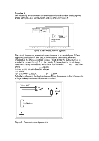
The resistivity measurement system that used was based on the four point
probe Schlumberger configuration and it is shown in figure 1
Figure 1 :The Measurement System
The circuit diagram of a constant current source is shown in figure 2.If we
apply input voltage Vin ,this circuit produces the same output current
irrespective the changes in load resistor Rload .Since the output current Io
equals the current through R on the resistor R,hence the the circuit shown
here has a nearly infinite load resistance. For Vin=0.6V and R=3000
ohms ……{given}
current Io can be calculated as follows
Io= Vin/R
Io= 0.6/3000 = 0.0002A or 0.2 mA
Actually by changing the load resistance Rload the opamp output changes its
voltage to keep the current Io remain constant.
Vin = 0.6V
Vload
R=3KOhm
Figure 2 : Constant current generator

2. Below is the table showing the values of Vload for different values of Rload for
the resistivity measurement system used i.e,Vin=0.6 V.
Rload(Ohms) V load (Volts) Io load(A)
1000 0.2 0.0002
2000 0.4 0.0002
3000 0.6 0.0002
4000 0.8 0.0002
5000 1 0.0002
6000 1.2 0.0002
Table showing results of Vload at Different Rload
Plotting graph between Vload and Rload we have got
Vload Vs Rload
1.4
1.2 y = 0.0002x
1
Vload (Vlots)
0.8 Series1
0.6 Linear (Series1)
0.4
0.2
0
0 5000 10000
Rload (ohms)
Graph between Vload Vs Rload
From the above graph between Vload and Rload the equation of line is given
by
Y=0.0002x
Where Gradient=Vload/Rload=Io
Therefore
Io=0.0002 A
Results:
From the graph we can see that the gradient remains the same for all values
of Rload.
Hence we can say that in this constant current source the output current Io is
independent of the changes in Rload and therefore the circuit has nearly
infinite load resistance within the compliance range.

3. .
Exercise 2:Measurement Strategies
Figure 1:Resistivity Measurement strategy used in archaeology site
The measuring system used in a archaeology site (as shown by figure 1) for
measuring electrical resistivity or conductivity of any material was based on
the four point probe method.This is a simple and low cost method which is
first proposed by Thomson in 1861 and first used by Schlumberger in 1920 to
measure the resistivity of Earth.
Principle
The basic principle of four point probe method is illustrated in the figure below
Ground
Four Point Probe Method
“By applying constant current to the outer electrodes ,Potential Difference can
be measured by the inner electrodes at different positions on the surface of
the material .The current remains constant in the circuit irrespective to the

4. changes in resistances and the output voltage is totally dependent on the
resistance changes.”
The four point method offers advantages over Direct or two probes method
which offer very poor performance due to polarization and electrode contact
issues. By using constant current source the current flowing through the
material will largely independent to the probe/contact impedances as current
remains constant as resistance changes.For verification below is the
experimental results showing that the current remains same for different
values of load resistances and only the output voltage will be changed with
resistance.this experiment was performed with 1 mA current source with
different values of resistances.and the output voltage of 15 V as opamp
maximum i/p was 15 V and the opamp saturated at 13 volts approximately.
R Vout I
ohms (volts) (amperes)
1000 1.02 0.00102
2000 2 0.001
3000 3.05 0.001017
4000 4.07 0.001018
5000 5.08 0.001016
6000 6.1 0.001017
7000 7.12 0.001017
8000 8.15 0.001019
9000 9.165 0.001018
10000 10.18 0.001018
11000 11.18 0.001016
12000 12.19 0.001016
13000 13.21 0.001016
Results from Laborator experiment for verification of constant current source
The graph between different Voltage and resistances values is shown below .

5. V vs R(Linear Range)
14
y = 0.0010x - 0.0050
12
10
8
Vo (V)
Linear
6 Linear (Linear)
4
2
0
0 5000 10000 15000
R(ohm)
Also to ensure that virtually no current will flow through the voltage measuring
electrodes an instrumentational amplifier is used as shown in the figure.
In designing the voltage measuring electrodes should be as near to resistance
as possible to minimize contact resistance and loading effects.
The current follows the path according to the distribution of resistivity within
the region.Thereore the potential difference between the two inner probes
contains the information about the distribution of electrical resistivity.
For measuring resistivity of the ground currents are injected into the ground
and the resulting potential differences are measured at the surface.The in situ
measurement of resistivity is impractical as it is the resistance measured
between the faces of a unit cube of material.Therefore the common method is
to measure the resistance on the surface of a material and then calculate the
apparent resistivity values using the current and voltage measurements and
the electrode configuration used
Mostly low frequency alternating sources are applied to the ground for
avoiding the polarization effect.
In practice the frequency of the alternating current required to penetrate in
the ground decreases with the increase in depth.
F a.c. α 1/depth
In general a frequency of 100 Hz is required to penetrate in 10m depth
whereas 10 Hz for 100m.
The resistivity for a conducting cylinder of resistance ∆R,length ∆L and cross
sectional area ∆A is given by:
=∆R ∆A/∆L ………eq(1)

6. Current Flow in the ground:
Consider a homogeneous material,when current I will flow through it it will
follow the radial pattern from the electrode and create hemispherical
equipotential surfaces.
From Ohms’s Law and substituting values in eq 1 we know that
∆V/∆L = I/∆A = - i …………………..eq(2)
The potential gradient ∆V/∆L is dependent on the current density I and the
resistivity of the material.
If the electrode is at distance r the surface area is 2πr² and hence current
density I is given by
i=I/2πr²
Now the potential gradient is given by
Equation (3)
Now the potential Vr at a distance r can be found by integerating above
equation (3)
The potential can be calculated at any point on or below the surface of a
homogeneous surface or ground by using above equation.
If the sink electrode is at a finite distance from the source as illustrated in the
figure below

7. The potential at any point is the sum of the potential contributions from each
current conducting electrode.
Absolute potential are difficult to measure hence normally the potential
difference ∆V between any two voltage sensing electrodes is measured and is
given by
By using the above equation the electric resistivity can be calculated for any
electrode configuration . The resistivity should be independent of the both
electrode spacing and geometery and same for a uniform material but if the
material is non uniform the electric resistivity will vary with the electrode
position.
Actually the apparent resistivity does not represent the average resistivity of
the material and hence negative values can be possible. It does however
provide a
means of scanning a region for resistivity variations and hence offers the
possibility of tomographic imaging. The depth of penetration of the current
increases as the separation of the current electrodes is increased and hence
it is possible to probe the material to different depths.
In general the depth of penetration is limited to about half the electrode
separation with features close to the surface having a greater influence on the
current path (MC Phillipson et. All)
Lock in Amplifier:
By using the lock-in amplifier the effects of noise can be subsequently
reduced and therefore it improves the signal to noise ratio. The main
advantages are that it responds to the frequency of interest, and the reference
frequency can be chosen to minimize the effect of 1/f and to avoid strong
interfering noise signals.Actually, the lock-in amplifier is a phase sensitive
detector which performs the following additional functions:
o Phase shifting of input signal with respect to reference signal
o Amplification and filtering of input signal.
o Narrow bandwidth detection

8. Exercise 3:
To calculate the apparent resistivity and by plotting the graph between
resistivity and position find out if there is any archaeological objects hidden
inside the ground.
Solution:
It is given that
Array (current injection probes) separation 2L =6.5 m
Voltage probes separation 2l=0.2 m
Injected current =0.0002 A
The provided data are illustrated in columns 1,2 of the following table.
Position of
mid point of
potential
electrodes
from LHS of
site. DVmeasured
(m) (V)
0.5 0.14
1.0 0.14
1.5 0.10
2.0 0.22
2.5 0.60
3.0 0.20
3.5 0.16
4.0 0.10
4.5 0.11
5.0 0.16
5.5 0.30
6.0 1.10
Since the distance ‘x between mid points of current and potential electrodes
Is not zero.Hence resistivity can be calculated using the formula:
π ( L2 − x 2 ) 2 ∆V
ρ= meters*Volts/Ampere
2l ( L2 − x 2 ) I
Where
L=3.25m,
2l=0.2m,
I=0.002A,
x=L –Potential Electrode (LHS position)

9. To calculate the distance ‘x’ and resistivity we used spreadsheet file and
below is the table showing the results
x'
Position of Distatanc
mid point of e from
potential the centre
electrodes of
from LHS of Electrode
site. DVmeasured s Resistivity
(m) (V) (m) Meter*V/A
0.5 0.14 2.75 545.987137
1.0 0.14 2.25 2128.743182
1.5 0.10 1.75 3242.469482
2.0 0.22 1.25 11542.92394
2.5 0.60 0.75 42358.55263
3.0 0.20 0.25 16299.32189
3.5 0.16 -0.25 13039.45751
4.0 0.10 -0.75 7059.758772
4.5 0.11 -1.25 5771.461968
5.0 0.16 -1.75 5187.951171
5.5 0.30 -2.25 4561.592533
6.0 1.10 -2.75 4289.898934
Table :Calculated Resistivity and distance x values from spreadsheet
The graph of the resistivity versus position is shown in figure 4.
Resistivity Vs Distance 'x'
45000
0.75, 42358.55263
40000
35000
30000
Resistivity
25000
Series1
20000
15000
10000
5000
0
-4 -3 -2 -1 0 1 2 3 4
Distance 'x'
Figure 1: Resistivity Vs Distance ‘x’
Results:
From the graph it is clear that between the region -0.25 to +1.25 there is a
change in the resistivity of the region and at distance around 0.75 m is a clear
indication of some changes in the layer composition.Actually electrical

10. resistivity of stones ,rocks and hydrocarbons are much higher than the
soil.Therefore between region of -0.25 to +1.25 there may be some valuable
archaeological objects hidden beneath the position.
Exercise 4:Vertical electrical sounding (VES)
Vertical electrical sounding or electrical drilling is a detailed method to find out
the information on the vertical succession of different conducting zones and
their individual thickness and true resistivity and the method is based on the
four point probe method.(Schlumberger array).(http://www.geo-
serv.de/geoelec_VES_water.html)
In order to achieve vertical electrical sounding the relative spacing between
the electrodes should be maintained same and the position of the electrodes
should be expanded over a central fixed point .
Actually by expanding the electrodes the electric field generated by the
injected current electrodes can be increased vertically or down the ground
and this method can be used to find the objects deeper inside the ground.The
technique can be describe by the following diagram.