Six Sigma Methods and Formulas for Successful Quality Management

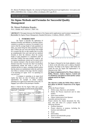
Dr. Maruti Prabhakar Rapaka. Int. Journal of Engineering Research and Application www.ijera.com
ISSN: 2248-9622, Vol. 7, Issue 1, (Part -5) January 2017, pp.49-52
www.ijera.com 49 | P a g e
Six Sigma Methods and Formulas for Successful Quality
Management
Dr. Maruti Prabhakar Rapaka
Ph.D., SSMBB, MCP, PRINCE 2, MSP, ITIL
ABSTRACT: This paper discusses the Methods of Six Sigma and its applications used in project management.
Keywords: Six Sigma, Project Management, Standard Deviation, 3.4 defects, DMAIC, ANOVA.
I. INTRODUCTION
Six Sigma is basically the application of
Statistical formulas and Methods to eliminate defects,
variation in a product or a process. For example if you
want to find the average height of male population in
India, you cannot bring the entire population of more
than 2 billion into one room and measure their height
for a scenario like this we take samples that is we pick
up sample(people) from each state and use statistical
formulas to draw the inference about the average
height of male population in a population which is
more than 2 billion. One more example would be say
a company manufactures pistons use d in motor cycles
the customer demand is that the piston should not a
diameter more than 9 cm and less than 5 cm anything
manufactured outside this limits is said to be a
variation and the six sigma consultant should confirm
that the pistons are manufactured within the said limits
else if there is variation in the range then the company
is not operating at 6 sigma level it is operating at a
very low level.
A company is operating at six sigma level
implies that there are only 3.4 defects per million
opportunities for example an airline company
operating at six sigma level means that it loses only 3.4
baggage’s per million of the passenger it handles.
Below is Shown the Six Sigma Table and a graph
explaining the meaning of various levels of Six Sigma.
Sigma Level Defect Rate Yield
Percentage
2 σ 308,770 dpmo (Defects Per
Million Opportunities)
69.10000 %
3 σ 66,811 dpmo 93.330000 %
4 σ 6,210 dpmo 99.38000 %
5 σ 233 dpmo 99.97700 %
6 σ 3.44 dpmo 99.99966 %
Six Sigma is Denoted by the Greek alphabet σ which
is shown in the table above and is called as Standard
deviation. The father of Six Sigma is Bill Smith who
coined the term Six Sigma and implemented it in
Motorola in the 1980’s.
Six Sigma is implemented in Five Phases which are
Define, Measure, Analyze, Improve, Control and
we will discuss each phases in brief and the various
methods used in Six Sigma.
Define
The objectives within the Define Phase which is
first phase in DMAIC framework of Six Sigma
are: -
Define the Project Charter
 Define scope, objectives, and schedule
 Define the Process (top-level) and its stake
holders
 Select team members
 Obtain Authorization from Sponsor
Assemble and train the team.
Project charters the charter documents the why,
how, who and when of a project include the
following elements
 Problem Statement
 Project objective or purpose, including the
business need addressed
 Scope
 Deliverables
 Sponsor and stakeholder groups
 Team members
RESEARCH ARTICLE OPEN ACCESS

 Project schedule (using GANTT or PERT as
an attachment)
 Other resources required
Work break down Structure
It is a process for defining the final and
intermediate products of a project and their
relationship. Defining Project task is typically
complex and accomplished by a series of
decomposition followed by a series of aggregations
it is also called top down approach and can be used
in the Define phase of Six Sigma framework.
Now we will get into the formulas of Six Sigma
which is shown in the table below.
Central tendency is defined as the tendency for
the values of a random variable to cluster round its
mean, mode, or median.
Central Tendency Population Sample
Mean/Average µ =∑ (Xi)^2/N XBar=∑
(Xi)^2/n
Median Middle value of Data
Most occurring value in the dataMode
Dispersion
Variance σ ^2 = ∑(X-
µ)^2/ N
S^2 = ∑(Xi-
XBar)^2/ n-1
Standard Deviation σ= ∑(Xi- µ)^2/
N
S = ∑(Xi-
XBar)^2/ n-1
Range Max-Min
Where mean is the average for example if
you have taken 10 sample of pistons randomly from
the factory and measured their diameter the average
would be sum of the diameter of the 10 pistons
divided by 10 where 10 the number of observations the
sum in statistics is denoted by ∑. In the above table X,
Xi are the measures of the diameter of the piston and
µ,X-Bar is the average.
Mode is the most frequently observed
measurement in the diameter of the piston that is if 2
pistons out 10 samples collected have the diameter as
6.3 & 6.3 then this is the mode of the sample and
median is the midpoint of the observations of the
diameter of the piston when arranged in sorted order.
From the example of the piston we find that
the formulas of mean, median, mode does not correctly
depict variation in the diameter of the piston
manufactured by the factory but standard deviation
formula helps us to find the variance in the diameter of
the piston manufactured which is varying from the
customer mentioned upper specification limit and
lower specification limit.
The most important equation of Six Sigma is
Y = f(x) where Y is the effect and x are the causes so if
you remove the causes you remove the effect of the
defect. For example, headache is the effect and the
causes are stress, eye strain, fever if you remove this
causes automatically the headache is removed this is
implemented in Six Sigma by using the Fishbone or
Ishikawa diagram invented by Dr Kaoru Ishikawa.
Measure Phase: In the Measure phase, we collect all
the data as per the relationship to the voice of customer
and relevantly analyze using statistical formulas as
given in the above table. Capability analyses is done in
measure phase.
The process capability is calculated using the
formula CP = USL-LSL/6 * Standard Deviation
where CP = process capability index, USL =
Upper Specification Limit and LSL = Lower
Specification Limit.
The Process capability measures indicates the
following
1. Process is fully capable
2. Process could fail at any time
3. Process is not capable.
When the process is spread well within the
customer specification the process is considered to
be fully capable that means the CP is more than
2.In this case, the process standard deviation is so
small that 6 times of the standard deviation with
reference to the means is within the customer
specification.
Example: The Specified limits for the diameter
of car tires are 15.6 for the upper limit and 15
for the lower limit with a process mean of 15.3
and a standard deviation of 0.09. FindCp and Cr
what can we say about Process Capabilities?
Cp= USL-LSL/ 6 * Standard deviation = 15.6 – 15
/ 6 * 0.09 = 0.6/0.54 = 1.111
Cp= 1.111
Cr = 1/ 1.111 = 0.9
Since Cp is greater than 1 and therefore Cr is less
than 1; we can conclude that the process is
potentially capable.
Analyze Phase:
In this Phase, we analyze all the data collected in the
measure phase and find the cause of variation. Analyze
phase use various tests like parametric tests where the
mean and standard deviation of the sample is known
and Nonparametric Tests where the data is categorical
for example as Excellent, Good, bad etc.
Parametric Hypothesis Test -A hypothesis is a
value judgment made about a circumstance, a
statement made about a population. Based on
experience an engineer can for instance assume that
the amount of carbon monoxide emitted by a
certain engine is twice the maximum allowed
legally. However, his assertions can only be
ascertained by conducting a test to compare the
carbon monoxide generated by the engine with the
legal requirements.
If the data used to make the comparison are
parametric data that is data that can be used to
derive the mean and the standard deviation, the

population from which the data are taken are
normally distributed they have equal variances. A
standard error based hypothesis testing using the t-
test can be used to test the validity of the
hypothesis made about the population. There are at
least 3 steps to follow when conducting hypothesis.
1. Null Hypothesis: The first step consists of
stating the null hypothesis which is the
hypothesis being tested. In the case of the
engineer making a statement about the level of
carbon monoxide generated by the engine, the
null hypothesis is
H0: the level of carbon monoxide generated by the
engine is twice as great as the legally required
amount. The Null hypothesis is denoted by H0
2. Alternate hypothesis: the alternate (or
alternative) hypothesis is the opposite of null
hypothesis. It is assumed valid when the null
hypothesis is rejected after testing. In the case
of the engineer testing the carbon monoxide
the alternative hypothesis would be
H1: The level of carbon monoxide generated by the
engine is not twice as great as the legally
required amount.
3. Testing the hypothesis: the objective of the test
is to generate a sample test statistic that can be
used to reject or fail to reject the null
hypothesis. The test statistic is derived from Z
formula if the samples are greater than 30.
Z = Xbar-µ/σ/ √n
If the samples are less than 30, then the t-test is
used
T= X bar -µ/ s/√n where X bar and µ is the mean
and s is the standard deviation.
1-Sample t Test (Mean v/s Target) this test is used
to compare the mean of a process with a target
value such as an ideal goal to determine whether
they differ it is often used to determine whether a
process is off center
1 Sample Standard Deviation This test is used to
compare the standard deviation of the process with
a target value such as a benchmark whether they
differ often used to evaluate how consistent a
process is
2 Sample T (Comparing 2 Means) Two sets of
different items are measured each under a different
condition there the measurements of one sample
are independent of the measurements of other
sample.
Paired T The same set of items is measured under
2 different conditions therefore the 2 measurements
of the same item are dependent or related to each
other.
2-Sample Standard This test is used when
comparing 2 standard deviations
Standard Deviation test This Test is used when
comparing more than 2 standard deviations
Non-Parametric hypothesis Tests are conducted
when data is categorical that is when the mean and
standard deviation are not known examples are
Chi-Square tests, Mann-Whitney U Test, Kruskal
Wallis tests & Moods Median Tests.
Anova
If for instance 3 sample means A, B, C are being
compared using the t-test is cumbersome for this
we can use analysis of variance ANOVA can be
used instead of multiple t-tests.
ANOVA is a Hypothesis test used when more than
2 means are being compared.
If K Samples are being tested the null hypothesis
will be in the form given below
H0: µ1 = µ2 = ….µk
And the alternate hypothesis will be
H1: At least one sample mean is different from the
others
If the data you are analyzing is not normal you have to
make it normal using box cox transformation to
remove any outliers (data not in sequence with the
collected data).Box Cox Transformation can be done
using the statistical software Minitab.
Improve Phase: In the Improve phase we focus on
the optimization of the process after the causes are
found in the analyze phase we use Design of
experiments to remove the junk factors which don’t
contribute to smooth working of the process that is in
the equation Y = f(X) we select only the X’s which
contribute to the optimal working of the process.
Let us consider the example of an
experimenter who is trying to optimize the
production of organic foods. After screening to
determine the factors that are significant for his
experiment he narrows the main factors that affect
the production of fruits to “light” and “water”. He
wants to optimize the time that it takes to produce
the fruits. He defines optimum as the minimum
time necessary to yield comestible fruits.
To conduct his experiment he runs several
tests combining the two factors (water and light) at
different levels. To minimize the cost of
experiments he decides to use only 2 levels of the
factors: high and low. In this case we will have two
factors and two levels therefore the number of runs
will be 2^2=4. After conducting observations he
obtains the results tabulated in the table below.
Factors Response
Water –High Light
High
10 days
Water high – Light low 20 days
Water low – Light high 15 days
Water low – Light low 25 days

Control Phase: In the Control phase we document all
the activities done in all the previous phases and using
control charts we monitor and control the phase just to
check that our process doesn’t go out of control.
Control Charts are tools used in Minitab Software to
keep a check on the variation. All the documentation
are kept and archived in a safe place for future
reference.
II. CONCLUSION
From the paper we come to understand that selection
of a Six Sigma Project is Critical because we have to
know the long term gains in executing these projects
and the activities done in each phase the basic building
block is the define phase where the problem statement
is captured and then in measure phase data is collected
systematically against this problem statement which is
further analyzed in Analyze phase by performing
various hypothesis tests and process optimization in
Improve phase by removing the junk factors that is in
the equation y = f(x1, x2,x3…….) we remove the
causes x1, x2 etc. by the method of Design of
Experiments and factorial methods. Finally we can
sustain and maintain our process to the optimum by
using control charts in Control Phase.
REFERENCES
[1] The Certified Master Black Belt Book By T. M
Kubiak.
[2] The Six Sigma Hand Book by : Thomas Pyzdek and
Paul Keller.

Six Sigma Methods and Formulas for Successful Quality Management

Recommandé

Recommandé

Contenu connexe

Tendances

Tendances (19)

En vedette

En vedette (20)

Similaire à Six Sigma Methods and Formulas for Successful Quality Management

Similaire à Six Sigma Methods and Formulas for Successful Quality Management (20)

Dernier

Dernier (20)

Six Sigma Methods and Formulas for Successful Quality Management