SlideShare une entreprise Scribd logo
1  sur  27
• Early ideas of decomposing a
periodic function into the sum of
simple oscillating functions date
back to the 3rd century BC.
• The Fourier series is named in
honour of Jean-Baptiste Joseph
Fourier (1768–1830), who made
important contributions to the
study of trigonometric series.
• Fourier introduced the series for
the purpose of solving the heat
equation in a metal plate,
publishing his initial results in his
1807 and publishing Analytical
theory of heat in 1822.
• The heat equation is a partial differential equation. Prior to
Fourier's work, no solution to the heat equation was known in
the general case, although particular solutions were known if
the heat source behaved in a simple way, in particular, if the
heat source was a sine or cosine wave.
• Fourier's idea was to model a complicated heat source as a
superposition (or linear combination) of simple sine and
cosine. This superposition or linear combination is called the
Fourier series.
• Although the original motivation was to solve the heat
equation, it later became obvious that the same techniques
could be applied to a wide array of mathematical and physical
problems.
Determining the
Fourier Series Representation of a
Continuous Time Signal
tjntjk
k
k
tjn
eeaetx 000
)(  




 1)( )/2(0





tTjk
k
k
tjk
k
k
eaeatx 
A periodic CT signal can be expressed as a linear combination of harmonically related
complex exponentials of the form :-
Multiplying both sides with , we get :-
tjn
e 0
Now if we integrate both sides from 0 to T, we have :-
dteeadtetx
T
tjntjk
k
k
T
tjn






00
000
)( 
Interchanging the order of integration and summation :-
 2)(
00
000






 




T
tjntjk
k
k
T
tjn
dteeadtetx 
Applying Euler’s formula to the bracketed Integral :-
 
TTT
tnkj
tdtnkjtdtnkdte
0
0
0
0
0
)(
)sin()cos(0



T
tnkj
dte
0
)( 0 T, if k = n
0, if k n{
In the R.H.S. side of the integral, for ‘k’ not equal to ‘n’, both the integrals will be zero.
Fr k=n, the integrand equals ‘1’ and thus, the integral equals ‘T’.


T
tnkj
dte
0
)( 0 T, if k = n
0, if k n{

dte
T
tnkj 0)( 
Integrating from 0 to T is same as integrating over any interval of length T because we
are only concerned with integral number of periods of cosine and sine function in the
previous equation.
Now the R.H.S. of equation (2) reduces to Tan . Therefore :-
dtetx
T
a
T
tjn
n 


0
0
)(
1 
Consequently, we can write
dtetx
T
a
T
tjn
n 

 0
)(
1 
Hence the Fourier series of x(t) can be expressed as :-
 
 4)(
1
)(
1
3)(
)/2(
)/2(
0
0








dtetx
T
dtetx
T
a
eaeatx
T
tTjk
T
tjk
k
tTjk
k
k
tjk
k
k


Here equation (3) is the analysis equation and equation (4) is the synthesis equation.
Coefficients ak are called Fourier Series Coefficients or Spectral Coefficients of x(t).
Here the DC or constant component of x(t) is :-
dttx
T
a
T

0
0 )(
1
7
Example :- Periodic square wave defined over one period as
 







2/tT0
t1
1
1
T
T
tx
1
 tx
-T -T/2 –T1 0 T1 T/2 T t
 
Defining
 10
1
sin
2
Tkc
T
T
ak 


k
Tk
ak
10sin
 When k 0
At k = 0  
T
T
dttx
T
a
T
T
1
2/
/2-
0
21
 

 
x
x
xc
sin
sin 
Fourier Series of some Common Signals
Conditions for convergence of
CT Fourier series
• Every function ƒ(x) of period 2п satisfying following conditions known as
DIRICHLET’S CONDITIONS, can be expressed in the form of Fourier series.
1. Over any period, x(t) must be absolutely integrable :-
it guarantees that each coefficient ak will be finite
2. In a single period, x(t) should have finite number of max and min
3. In any finite interval of time, there are only a finite number of discontinuities. Each
discontinuity should be finite.
 dttx
T
2
)(
ka
Properties of CT Fourier Series
1. Linearity
z(t) = Ax(t) + By(t) ck = Aak + Bbk
2. Time Shifting
z(t) = x(t-t0) ck =
• In time shifting magnitude of Fourier series coefficient remains the same
|ck| = |ak|
3. Time Reversal
z(t) = x(-t) ck = a-k
• If x(t) is even, ak = a-k
• If x(t) is odd, ak = -a-k
x(t) & y(t) are two periodic signals with period T and
Fourier coefficients ak & bk respectively
00tjk
k ea 
4. Time Scaling
z(t) = x(αt) ck = ak
• But, the fundamental period is (T/α)
5. Multiplication
z(t) = x(t)y(t) ck =
• (DT convolution between coefficients)
6. Conjugation & Conjugate Symmetry
• Real x(t) a-k = a*k (conjugate symmetric)
• Real & Even x(t) ak = a*k (real & even ak)
• Real & Odd x(t) ak = -a*k (purely imaginary & odd ak ; a0 = 0)
• z(t) = Even part of x(t) ck = Real{ak}
• z(t) = Odd part of x(t) ck = jImaginary{ak}




l
lklba
7. Periodic Convolution
8. Parseval’s Relation
• Total average power = sum of average power in all harmonic components
• Energy in time domain equals to energy in frequency domain
 dtyxtytx
T
)()()(*)(   Takbk

 








k
k
T
tjk
k
k
T k
tjk
k
T
adtea
T
dtea
T
dttx
T
222
2
2
0
0
1
1
)(
1


Determining the
Fourier Series Representation of a
Discrete Time Signal
 1][ )/2(0
   Nk
nNjk
k
Nk
njk
k eaeanx 
A periodic DT signal can be expressed as set of N linear equations for N unknown
coeffficients ak as k ranges over a set of N successive integers :-
Nn
nNjk
e )/2(  N, if k = 0,+N,+2N…
0, otherwise
{
According to the fact that :-



Nk
nNrkj
k
nNjr
eaenx )/2)(()/2(
][ 
Multiplying both sides with , we get :-
nNjr
e )/2( 
Now if summing over N terms, we have :-
   




Nn Nk
nNrkj
k
Nn
nNjr
eaenx )/2)(()/2(
][ 
Interchanging the order of summation, we have :-
   




Nk Nn
nNrkj
k
Nn
nNjr
eaenx )/2)(()/2(
][ 


Nn
nNrkj
e )/2)((  N, if k = 0,+N,+2N…
0, otherwise
{
According to the fact stated before, we can conclude that :-
So the R.H.S. of the equation reduces to Nar



Nn
nNjr
r enx
N
a )/2(
][
1 
Hence the Fourier series of x[n] can be expressed as below where equation (3) is the
analysis equation and equation (4) is the synthesis equation
 
 4][
1
][
1
3][
)/2(
)/2(
0
0









Nn
nNjk
Nn
njk
k
Nk
nNjk
k
Nk
njk
k
enx
N
enx
N
a
eaeanx


Properties of DT Fourier Series
1. Linearity
z[n] = Ax[n] + By[t] ck = Aak + Bbk
2. Time Shifting
z[t] = x[n-n0] ck =
• In time shifting magnitude of Fourier series coefficient remains the same
|ck| = |ak|
3. Time Reversal
z[t] = x[-n] ck = a-k
• If x[n] is even, ak = a-k
• If x[n] is odd, ak = -a-k
x[n] & y[n] are two periodic signals with period N and
Fourier coefficients ak & bk respectively periodic with period N
0)/2( nNjk
k ea 
4. Multiplication
z[n] = x[n]y[n] ck =
5. Conjugation & Conjugate Symmetry
• Real x[n] a-k = a*k (conjugate symmetric)
• Real & Even x[n] ak = a*k (real & even ak)
• Real & Odd x[n] ak = -a*k (purely imaginary & odd ak )
• z[n] = Even part of x[n] ck = Real{ak}
• z[n] = Odd part of x[n] ck = jImaginary{ak}
6. Periodic Convolution


Nl
lklba


Nr
rnyrxnynx ][][][*][ Nakbk
7. Parseval’s Relation
• Total average power = sum of average power in all harmonic components
• Energy in time domain equals to energy in frequency domain
22
][
1
 

Nk
k
Nn
anx
N
FOURIER SERIES, which is an infinite series representation of such
functions in terms of ‘sine’ and ‘cosine’ terms, is useful here. Thus,
FOURIER SERIES, are in certain sense, more UNIVERSAL than TAYLOR’s
SERIES as it applies to all continuous, periodic functions and also to the
functions which are discontinuous in their values and derivatives.
FOURIER SERIES a very powerful method to solve ordinary and partial
differential equation..
As we know that TAYLOR SERIES representation of functions are valid
only for those functions which are continuous and differentiable. But
there are many discontinuous periodic function which requires to
express in terms of an infinite series containing ‘sine’ and ‘cosine’
terms.
Advantages of using Fourier Series
Consider a mass-spring system as before, where we have a mass m on a
spring with spring
constant k, with damping c, and a force F(t) applied to the mass.
Suppose the forcing function F(t) is 2L-periodic for some
L > 0.
The equation that governs this
particular setup is
The general solution consists of the
complementary solution xc, which
solves the associated
homogeneous equation mx” + cx’ + kx = 0, and a particular solution of (1)
we call xp.
mx”(t) + cx’(t) + kx(t) = F(t)
Applications of using Fourier Series
1. Forced Oscillation
For c > 0,
the complementary solution xc will decay as time goes by. Therefore, we
are mostly interested in a
particular solution xp that does not decay and is periodic with the same
period as F(t). We call this
particular solution the steady periodic solution and we write it as xsp as
before. What will be new in
this section is that we consider an arbitrary forcing function F(t) instead of
a simple cosine.
For simplicity, let us suppose that c = 0. The problem with c > 0 is very
similar. The equation
mx” + kx = 0
has the general solution,
x(t) = A cos(ωt) + B sin(ωt);
Where,
Any solution to mx”(t) + kx(t) = F(t) is of the form
A cos(ωt) + B sin(ωt) + xsp.
The steady periodic solution xsp has the same period as F(t).
In the spirit of the last section and the idea of undetermined
coefficients we first write,
Then we write a proposed steady periodic solution x as,
where an and bn are unknowns. We plug x into the deferential
equation and solve for an and bn in terms of cn and dn.
• It turns out that (almost) any kind of a wave can be written as a sum of sines and
cosines. So for example, if a voice is recorded for one second saying something, I
can find its Fourier series which may look something like this for example
• and this interactive module shows you how when you add sines and/or cosines the
graph of cosines and sines becomes closer and closer to the original graph we are
trying to approximate.
• The really cool thing about Fourier series is that first, almost any kind of a wave
can be approximated. Second, when Fourier series converge, they converge very
fast.
• So one of many applications is compression. Everyone's favorite MP3 format uses
this for audio compression. You take a sound, expand its Fourier series. It'll most
likely be an infinite series BUT it converges so fast that taking the first few terms is
enough to reproduce the original sound. The rest of the terms can be ignored
because they add so little that a human ear can likely tell no difference. So I just
save the first few terms and then use them to reproduce the sound whenever I
want to listen to it and it takes much less memory.
• JPEG for pictures is the same idea.
2. Speech/Music Recognition
3. Approximation Theory :- We use Fourier series to write a
function as a trigonometric polynomial.
4. Control Theory :- The Fourier series of functions in the
differential equation often gives some prediction about the
behavior of the solution of differential equation. They are
useful to find out the dynamics of the solution.
5. Partial Differential equation :- We use it to solve higher order
partial differential equations by the method of separation of
variables.

Contenu connexe

Tendances

Fir filter design (windowing technique)
Fir filter design (windowing technique)Fir filter design (windowing technique)
Fir filter design (windowing technique)
Bin Biny Bino
 
discrete time signals and systems
 discrete time signals and systems  discrete time signals and systems
discrete time signals and systems
Zlatan Ahmadovic
 

Tendances (20)

Digital Signal Processing[ECEG-3171]-Ch1_L02
Digital Signal Processing[ECEG-3171]-Ch1_L02Digital Signal Processing[ECEG-3171]-Ch1_L02
Digital Signal Processing[ECEG-3171]-Ch1_L02
 
Discrete Fourier Series | Discrete Fourier Transform | Discrete Time Fourier ...
Discrete Fourier Series | Discrete Fourier Transform | Discrete Time Fourier ...Discrete Fourier Series | Discrete Fourier Transform | Discrete Time Fourier ...
Discrete Fourier Series | Discrete Fourier Transform | Discrete Time Fourier ...
 
inverse z-transform ppt
inverse z-transform pptinverse z-transform ppt
inverse z-transform ppt
 
Chapter4 - The Continuous-Time Fourier Transform
Chapter4 - The Continuous-Time Fourier TransformChapter4 - The Continuous-Time Fourier Transform
Chapter4 - The Continuous-Time Fourier Transform
 
Sampling theorem
Sampling theoremSampling theorem
Sampling theorem
 
Chapter2 - Linear Time-Invariant System
Chapter2 - Linear Time-Invariant SystemChapter2 - Linear Time-Invariant System
Chapter2 - Linear Time-Invariant System
 
Z transform
Z transformZ transform
Z transform
 
DSP_2018_FOEHU - Lec 08 - The Discrete Fourier Transform
DSP_2018_FOEHU - Lec 08 - The Discrete Fourier TransformDSP_2018_FOEHU - Lec 08 - The Discrete Fourier Transform
DSP_2018_FOEHU - Lec 08 - The Discrete Fourier Transform
 
Dif fft
Dif fftDif fft
Dif fft
 
Discrete Time Fourier Transform
Discrete Time Fourier TransformDiscrete Time Fourier Transform
Discrete Time Fourier Transform
 
Fast fourier transform
Fast fourier transformFast fourier transform
Fast fourier transform
 
5. convolution and correlation of discrete time signals
5. convolution and correlation of discrete time signals 5. convolution and correlation of discrete time signals
5. convolution and correlation of discrete time signals
 
DSP_2018_FOEHU - Lec 04 - The z-Transform
DSP_2018_FOEHU - Lec 04 - The z-TransformDSP_2018_FOEHU - Lec 04 - The z-Transform
DSP_2018_FOEHU - Lec 04 - The z-Transform
 
Z Transform And Inverse Z Transform - Signal And Systems
Z Transform And Inverse Z Transform - Signal And SystemsZ Transform And Inverse Z Transform - Signal And Systems
Z Transform And Inverse Z Transform - Signal And Systems
 
Properties of dft
Properties of dftProperties of dft
Properties of dft
 
Solvedproblems 120406031331-phpapp01
Solvedproblems 120406031331-phpapp01Solvedproblems 120406031331-phpapp01
Solvedproblems 120406031331-phpapp01
 
Fir filter design (windowing technique)
Fir filter design (windowing technique)Fir filter design (windowing technique)
Fir filter design (windowing technique)
 
DSP_FOEHU - MATLAB 02 - The Discrete-time Fourier Analysis
DSP_FOEHU - MATLAB 02 - The Discrete-time Fourier AnalysisDSP_FOEHU - MATLAB 02 - The Discrete-time Fourier Analysis
DSP_FOEHU - MATLAB 02 - The Discrete-time Fourier Analysis
 
discrete time signals and systems
 discrete time signals and systems  discrete time signals and systems
discrete time signals and systems
 
Chapter3 - Fourier Series Representation of Periodic Signals
Chapter3 - Fourier Series Representation of Periodic SignalsChapter3 - Fourier Series Representation of Periodic Signals
Chapter3 - Fourier Series Representation of Periodic Signals
 

En vedette (8)

lte physical layer overview
 lte physical layer overview lte physical layer overview
lte physical layer overview
 
The Fast Fourier Transform (FFT)
The Fast Fourier Transform (FFT)The Fast Fourier Transform (FFT)
The Fast Fourier Transform (FFT)
 
Representation of complex number
Representation of complex numberRepresentation of complex number
Representation of complex number
 
Fft
FftFft
Fft
 
Properties of Fourier transform
Properties of Fourier transformProperties of Fourier transform
Properties of Fourier transform
 
1. introduction to complex numbers
1. introduction to complex numbers1. introduction to complex numbers
1. introduction to complex numbers
 
LTE Basics - II
LTE Basics - IILTE Basics - II
LTE Basics - II
 
Fast Fourier Transform
Fast Fourier TransformFast Fourier Transform
Fast Fourier Transform
 

Similaire à Fourier Series for Continuous Time & Discrete Time Signals

Find the compact trigonometric Fourier series for the periodic signal.pdf
Find the compact trigonometric Fourier series for the periodic signal.pdfFind the compact trigonometric Fourier series for the periodic signal.pdf
Find the compact trigonometric Fourier series for the periodic signal.pdf
arihantelectronics
 
torsionbinormalnotes
torsionbinormalnotestorsionbinormalnotes
torsionbinormalnotes
Jeremy Lane
 
Clarke fourier theory(62s)
Clarke   fourier theory(62s)Clarke   fourier theory(62s)
Clarke fourier theory(62s)
apsitachi
 

Similaire à Fourier Series for Continuous Time & Discrete Time Signals (20)

Fourier series
Fourier seriesFourier series
Fourier series
 
Fourier series
Fourier seriesFourier series
Fourier series
 
Fourier transform
Fourier transformFourier transform
Fourier transform
 
The wave equation
The wave equationThe wave equation
The wave equation
 
forrier serries.pptx
forrier serries.pptxforrier serries.pptx
forrier serries.pptx
 
Find the compact trigonometric Fourier series for the periodic signal.pdf
Find the compact trigonometric Fourier series for the periodic signal.pdfFind the compact trigonometric Fourier series for the periodic signal.pdf
Find the compact trigonometric Fourier series for the periodic signal.pdf
 
M220w07
M220w07M220w07
M220w07
 
Maths 3 ppt
Maths 3 pptMaths 3 ppt
Maths 3 ppt
 
Basic Introduction to Algebraic Geometry
Basic Introduction to Algebraic GeometryBasic Introduction to Algebraic Geometry
Basic Introduction to Algebraic Geometry
 
Nt lecture skm-iiit-bh
Nt lecture skm-iiit-bhNt lecture skm-iiit-bh
Nt lecture skm-iiit-bh
 
APPLICATION OF HIGHER ORDER DIFFERENTIAL EQUATIONS
APPLICATION OF HIGHER ORDER DIFFERENTIAL EQUATIONSAPPLICATION OF HIGHER ORDER DIFFERENTIAL EQUATIONS
APPLICATION OF HIGHER ORDER DIFFERENTIAL EQUATIONS
 
Dynamical systems solved ex
Dynamical systems solved exDynamical systems solved ex
Dynamical systems solved ex
 
Statistics Homework Help
Statistics Homework HelpStatistics Homework Help
Statistics Homework Help
 
Multiple Linear Regression Homework Help
Multiple Linear Regression Homework HelpMultiple Linear Regression Homework Help
Multiple Linear Regression Homework Help
 
torsionbinormalnotes
torsionbinormalnotestorsionbinormalnotes
torsionbinormalnotes
 
Statistica theromodynamics
Statistica theromodynamicsStatistica theromodynamics
Statistica theromodynamics
 
Clarke fourier theory(62s)
Clarke   fourier theory(62s)Clarke   fourier theory(62s)
Clarke fourier theory(62s)
 
Ch4 (1)_fourier series, fourier transform
Ch4 (1)_fourier series, fourier transformCh4 (1)_fourier series, fourier transform
Ch4 (1)_fourier series, fourier transform
 
Thermal diffusivity
Thermal diffusivityThermal diffusivity
Thermal diffusivity
 
Signals Processing Homework Help
Signals Processing Homework HelpSignals Processing Homework Help
Signals Processing Homework Help
 

Plus de Jayanshu Gundaniya

Engineering Mathematics - Total derivatives, chain rule and derivative of imp...
Engineering Mathematics - Total derivatives, chain rule and derivative of imp...Engineering Mathematics - Total derivatives, chain rule and derivative of imp...
Engineering Mathematics - Total derivatives, chain rule and derivative of imp...
Jayanshu Gundaniya
 

Plus de Jayanshu Gundaniya (15)

Erbium Doped Fiber Amplifier (EDFA)
Erbium Doped Fiber Amplifier (EDFA)Erbium Doped Fiber Amplifier (EDFA)
Erbium Doped Fiber Amplifier (EDFA)
 
Three Phase to Three phase Cycloconverter
Three Phase to Three phase CycloconverterThree Phase to Three phase Cycloconverter
Three Phase to Three phase Cycloconverter
 
Comparison of A, B & C Power Amplifiers
Comparison of A, B & C Power AmplifiersComparison of A, B & C Power Amplifiers
Comparison of A, B & C Power Amplifiers
 
Multiplexers & Demultiplexers
Multiplexers & DemultiplexersMultiplexers & Demultiplexers
Multiplexers & Demultiplexers
 
Initial Conditions of Resistor, Inductor & Capacitor
Initial Conditions of Resistor, Inductor & CapacitorInitial Conditions of Resistor, Inductor & Capacitor
Initial Conditions of Resistor, Inductor & Capacitor
 
First order non-linear partial differential equation & its applications
First order non-linear partial differential equation & its applicationsFirst order non-linear partial differential equation & its applications
First order non-linear partial differential equation & its applications
 
Engineering Mathematics - Total derivatives, chain rule and derivative of imp...
Engineering Mathematics - Total derivatives, chain rule and derivative of imp...Engineering Mathematics - Total derivatives, chain rule and derivative of imp...
Engineering Mathematics - Total derivatives, chain rule and derivative of imp...
 
Engineering Graphics - Projection of points and lines
Engineering Graphics - Projection of points and linesEngineering Graphics - Projection of points and lines
Engineering Graphics - Projection of points and lines
 
Internal expanding shoe brake short presentation
Internal expanding shoe brake short presentationInternal expanding shoe brake short presentation
Internal expanding shoe brake short presentation
 
Hydrological cycle
Hydrological cycleHydrological cycle
Hydrological cycle
 
Ecology and ecosystem
Ecology and ecosystemEcology and ecosystem
Ecology and ecosystem
 
Basics of pointer, pointer expressions, pointer to pointer and pointer in fun...
Basics of pointer, pointer expressions, pointer to pointer and pointer in fun...Basics of pointer, pointer expressions, pointer to pointer and pointer in fun...
Basics of pointer, pointer expressions, pointer to pointer and pointer in fun...
 
Architectural acoustics topics and remedies - short presentation
Architectural acoustics   topics and remedies - short presentationArchitectural acoustics   topics and remedies - short presentation
Architectural acoustics topics and remedies - short presentation
 
Superconductors and Superconductivity
Superconductors and SuperconductivitySuperconductors and Superconductivity
Superconductors and Superconductivity
 
Superposition theorem
Superposition theoremSuperposition theorem
Superposition theorem
 

Dernier

Standard vs Custom Battery Packs - Decoding the Power Play
Standard vs Custom Battery Packs - Decoding the Power PlayStandard vs Custom Battery Packs - Decoding the Power Play
Standard vs Custom Battery Packs - Decoding the Power Play
Epec Engineered Technologies
 
XXXXXXXXXXXXXXXXXXXXXXXXXXXXXXXXXXXXXXXXXXXXXXXXXXXX
XXXXXXXXXXXXXXXXXXXXXXXXXXXXXXXXXXXXXXXXXXXXXXXXXXXXXXXXXXXXXXXXXXXXXXXXXXXXXXXXXXXXXXXXXXXXXXXXXXXXXXXX
XXXXXXXXXXXXXXXXXXXXXXXXXXXXXXXXXXXXXXXXXXXXXXXXXXXX
ssuser89054b
 
"Lesotho Leaps Forward: A Chronicle of Transformative Developments"
"Lesotho Leaps Forward: A Chronicle of Transformative Developments""Lesotho Leaps Forward: A Chronicle of Transformative Developments"
"Lesotho Leaps Forward: A Chronicle of Transformative Developments"
mphochane1998
 
DeepFakes presentation : brief idea of DeepFakes
DeepFakes presentation : brief idea of DeepFakesDeepFakes presentation : brief idea of DeepFakes
DeepFakes presentation : brief idea of DeepFakes
MayuraD1
 

Dernier (20)

Standard vs Custom Battery Packs - Decoding the Power Play
Standard vs Custom Battery Packs - Decoding the Power PlayStandard vs Custom Battery Packs - Decoding the Power Play
Standard vs Custom Battery Packs - Decoding the Power Play
 
Engineering Drawing focus on projection of planes
Engineering Drawing focus on projection of planesEngineering Drawing focus on projection of planes
Engineering Drawing focus on projection of planes
 
XXXXXXXXXXXXXXXXXXXXXXXXXXXXXXXXXXXXXXXXXXXXXXXXXXXX
XXXXXXXXXXXXXXXXXXXXXXXXXXXXXXXXXXXXXXXXXXXXXXXXXXXXXXXXXXXXXXXXXXXXXXXXXXXXXXXXXXXXXXXXXXXXXXXXXXXXXXXX
XXXXXXXXXXXXXXXXXXXXXXXXXXXXXXXXXXXXXXXXXXXXXXXXXXXX
 
"Lesotho Leaps Forward: A Chronicle of Transformative Developments"
"Lesotho Leaps Forward: A Chronicle of Transformative Developments""Lesotho Leaps Forward: A Chronicle of Transformative Developments"
"Lesotho Leaps Forward: A Chronicle of Transformative Developments"
 
Computer Lecture 01.pptxIntroduction to Computers
Computer Lecture 01.pptxIntroduction to ComputersComputer Lecture 01.pptxIntroduction to Computers
Computer Lecture 01.pptxIntroduction to Computers
 
Thermal Engineering-R & A / C - unit - V
Thermal Engineering-R & A / C - unit - VThermal Engineering-R & A / C - unit - V
Thermal Engineering-R & A / C - unit - V
 
COST-EFFETIVE and Energy Efficient BUILDINGS ptx
COST-EFFETIVE  and Energy Efficient BUILDINGS ptxCOST-EFFETIVE  and Energy Efficient BUILDINGS ptx
COST-EFFETIVE and Energy Efficient BUILDINGS ptx
 
A CASE STUDY ON CERAMIC INDUSTRY OF BANGLADESH.pptx
A CASE STUDY ON CERAMIC INDUSTRY OF BANGLADESH.pptxA CASE STUDY ON CERAMIC INDUSTRY OF BANGLADESH.pptx
A CASE STUDY ON CERAMIC INDUSTRY OF BANGLADESH.pptx
 
Thermal Engineering -unit - III & IV.ppt
Thermal Engineering -unit - III & IV.pptThermal Engineering -unit - III & IV.ppt
Thermal Engineering -unit - III & IV.ppt
 
Online electricity billing project report..pdf
Online electricity billing project report..pdfOnline electricity billing project report..pdf
Online electricity billing project report..pdf
 
DC MACHINE-Motoring and generation, Armature circuit equation
DC MACHINE-Motoring and generation, Armature circuit equationDC MACHINE-Motoring and generation, Armature circuit equation
DC MACHINE-Motoring and generation, Armature circuit equation
 
Block diagram reduction techniques in control systems.ppt
Block diagram reduction techniques in control systems.pptBlock diagram reduction techniques in control systems.ppt
Block diagram reduction techniques in control systems.ppt
 
Hostel management system project report..pdf
Hostel management system project report..pdfHostel management system project report..pdf
Hostel management system project report..pdf
 
Introduction to Serverless with AWS Lambda
Introduction to Serverless with AWS LambdaIntroduction to Serverless with AWS Lambda
Introduction to Serverless with AWS Lambda
 
HAND TOOLS USED AT ELECTRONICS WORK PRESENTED BY KOUSTAV SARKAR
HAND TOOLS USED AT ELECTRONICS WORK PRESENTED BY KOUSTAV SARKARHAND TOOLS USED AT ELECTRONICS WORK PRESENTED BY KOUSTAV SARKAR
HAND TOOLS USED AT ELECTRONICS WORK PRESENTED BY KOUSTAV SARKAR
 
Tamil Call Girls Bhayandar WhatsApp +91-9930687706, Best Service
Tamil Call Girls Bhayandar WhatsApp +91-9930687706, Best ServiceTamil Call Girls Bhayandar WhatsApp +91-9930687706, Best Service
Tamil Call Girls Bhayandar WhatsApp +91-9930687706, Best Service
 
DeepFakes presentation : brief idea of DeepFakes
DeepFakes presentation : brief idea of DeepFakesDeepFakes presentation : brief idea of DeepFakes
DeepFakes presentation : brief idea of DeepFakes
 
Wadi Rum luxhotel lodge Analysis case study.pptx
Wadi Rum luxhotel lodge Analysis case study.pptxWadi Rum luxhotel lodge Analysis case study.pptx
Wadi Rum luxhotel lodge Analysis case study.pptx
 
FEA Based Level 3 Assessment of Deformed Tanks with Fluid Induced Loads
FEA Based Level 3 Assessment of Deformed Tanks with Fluid Induced LoadsFEA Based Level 3 Assessment of Deformed Tanks with Fluid Induced Loads
FEA Based Level 3 Assessment of Deformed Tanks with Fluid Induced Loads
 
NO1 Top No1 Amil Baba In Azad Kashmir, Kashmir Black Magic Specialist Expert ...
NO1 Top No1 Amil Baba In Azad Kashmir, Kashmir Black Magic Specialist Expert ...NO1 Top No1 Amil Baba In Azad Kashmir, Kashmir Black Magic Specialist Expert ...
NO1 Top No1 Amil Baba In Azad Kashmir, Kashmir Black Magic Specialist Expert ...
 

Fourier Series for Continuous Time & Discrete Time Signals

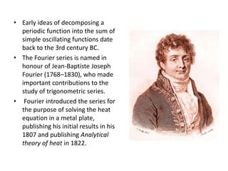
  • 1. • Early ideas of decomposing a periodic function into the sum of simple oscillating functions date back to the 3rd century BC. • The Fourier series is named in honour of Jean-Baptiste Joseph Fourier (1768–1830), who made important contributions to the study of trigonometric series. • Fourier introduced the series for the purpose of solving the heat equation in a metal plate, publishing his initial results in his 1807 and publishing Analytical theory of heat in 1822.
  • 2. • The heat equation is a partial differential equation. Prior to Fourier's work, no solution to the heat equation was known in the general case, although particular solutions were known if the heat source behaved in a simple way, in particular, if the heat source was a sine or cosine wave. • Fourier's idea was to model a complicated heat source as a superposition (or linear combination) of simple sine and cosine. This superposition or linear combination is called the Fourier series. • Although the original motivation was to solve the heat equation, it later became obvious that the same techniques could be applied to a wide array of mathematical and physical problems.
  • 3. Determining the Fourier Series Representation of a Continuous Time Signal tjntjk k k tjn eeaetx 000 )(        1)( )/2(0      tTjk k k tjk k k eaeatx  A periodic CT signal can be expressed as a linear combination of harmonically related complex exponentials of the form :- Multiplying both sides with , we get :- tjn e 0 Now if we integrate both sides from 0 to T, we have :- dteeadtetx T tjntjk k k T tjn       00 000 )( 
  • 4. Interchanging the order of integration and summation :-  2)( 00 000             T tjntjk k k T tjn dteeadtetx  Applying Euler’s formula to the bracketed Integral :-   TTT tnkj tdtnkjtdtnkdte 0 0 0 0 0 )( )sin()cos(0    T tnkj dte 0 )( 0 T, if k = n 0, if k n{ In the R.H.S. side of the integral, for ‘k’ not equal to ‘n’, both the integrals will be zero. Fr k=n, the integrand equals ‘1’ and thus, the integral equals ‘T’.
  • 5.   T tnkj dte 0 )( 0 T, if k = n 0, if k n{  dte T tnkj 0)(  Integrating from 0 to T is same as integrating over any interval of length T because we are only concerned with integral number of periods of cosine and sine function in the previous equation. Now the R.H.S. of equation (2) reduces to Tan . Therefore :- dtetx T a T tjn n    0 0 )( 1  Consequently, we can write dtetx T a T tjn n    0 )( 1 
  • 6. Hence the Fourier series of x(t) can be expressed as :-    4)( 1 )( 1 3)( )/2( )/2( 0 0         dtetx T dtetx T a eaeatx T tTjk T tjk k tTjk k k tjk k k   Here equation (3) is the analysis equation and equation (4) is the synthesis equation. Coefficients ak are called Fourier Series Coefficients or Spectral Coefficients of x(t). Here the DC or constant component of x(t) is :- dttx T a T  0 0 )( 1
  • 7. 7 Example :- Periodic square wave defined over one period as          2/tT0 t1 1 1 T T tx 1  tx -T -T/2 –T1 0 T1 T/2 T t   Defining  10 1 sin 2 Tkc T T ak    k Tk ak 10sin  When k 0 At k = 0   T T dttx T a T T 1 2/ /2- 0 21      x x xc sin sin 
  • 8. Fourier Series of some Common Signals
  • 9.
  • 10.
  • 11.
  • 12. Conditions for convergence of CT Fourier series • Every function ƒ(x) of period 2п satisfying following conditions known as DIRICHLET’S CONDITIONS, can be expressed in the form of Fourier series. 1. Over any period, x(t) must be absolutely integrable :- it guarantees that each coefficient ak will be finite 2. In a single period, x(t) should have finite number of max and min 3. In any finite interval of time, there are only a finite number of discontinuities. Each discontinuity should be finite.  dttx T 2 )( ka
  • 13. Properties of CT Fourier Series 1. Linearity z(t) = Ax(t) + By(t) ck = Aak + Bbk 2. Time Shifting z(t) = x(t-t0) ck = • In time shifting magnitude of Fourier series coefficient remains the same |ck| = |ak| 3. Time Reversal z(t) = x(-t) ck = a-k • If x(t) is even, ak = a-k • If x(t) is odd, ak = -a-k x(t) & y(t) are two periodic signals with period T and Fourier coefficients ak & bk respectively 00tjk k ea 
  • 14. 4. Time Scaling z(t) = x(αt) ck = ak • But, the fundamental period is (T/α) 5. Multiplication z(t) = x(t)y(t) ck = • (DT convolution between coefficients) 6. Conjugation & Conjugate Symmetry • Real x(t) a-k = a*k (conjugate symmetric) • Real & Even x(t) ak = a*k (real & even ak) • Real & Odd x(t) ak = -a*k (purely imaginary & odd ak ; a0 = 0) • z(t) = Even part of x(t) ck = Real{ak} • z(t) = Odd part of x(t) ck = jImaginary{ak}     l lklba
  • 15. 7. Periodic Convolution 8. Parseval’s Relation • Total average power = sum of average power in all harmonic components • Energy in time domain equals to energy in frequency domain  dtyxtytx T )()()(*)(   Takbk            k k T tjk k k T k tjk k T adtea T dtea T dttx T 222 2 2 0 0 1 1 )( 1  
  • 16. Determining the Fourier Series Representation of a Discrete Time Signal  1][ )/2(0    Nk nNjk k Nk njk k eaeanx  A periodic DT signal can be expressed as set of N linear equations for N unknown coeffficients ak as k ranges over a set of N successive integers :- Nn nNjk e )/2(  N, if k = 0,+N,+2N… 0, otherwise { According to the fact that :-
  • 17.    Nk nNrkj k nNjr eaenx )/2)(()/2( ][  Multiplying both sides with , we get :- nNjr e )/2(  Now if summing over N terms, we have :-         Nn Nk nNrkj k Nn nNjr eaenx )/2)(()/2( ][  Interchanging the order of summation, we have :-         Nk Nn nNrkj k Nn nNjr eaenx )/2)(()/2( ][ 
  • 18.   Nn nNrkj e )/2)((  N, if k = 0,+N,+2N… 0, otherwise { According to the fact stated before, we can conclude that :- So the R.H.S. of the equation reduces to Nar    Nn nNjr r enx N a )/2( ][ 1  Hence the Fourier series of x[n] can be expressed as below where equation (3) is the analysis equation and equation (4) is the synthesis equation    4][ 1 ][ 1 3][ )/2( )/2( 0 0          Nn nNjk Nn njk k Nk nNjk k Nk njk k enx N enx N a eaeanx  
  • 19. Properties of DT Fourier Series 1. Linearity z[n] = Ax[n] + By[t] ck = Aak + Bbk 2. Time Shifting z[t] = x[n-n0] ck = • In time shifting magnitude of Fourier series coefficient remains the same |ck| = |ak| 3. Time Reversal z[t] = x[-n] ck = a-k • If x[n] is even, ak = a-k • If x[n] is odd, ak = -a-k x[n] & y[n] are two periodic signals with period N and Fourier coefficients ak & bk respectively periodic with period N 0)/2( nNjk k ea 
  • 20. 4. Multiplication z[n] = x[n]y[n] ck = 5. Conjugation & Conjugate Symmetry • Real x[n] a-k = a*k (conjugate symmetric) • Real & Even x[n] ak = a*k (real & even ak) • Real & Odd x[n] ak = -a*k (purely imaginary & odd ak ) • z[n] = Even part of x[n] ck = Real{ak} • z[n] = Odd part of x[n] ck = jImaginary{ak} 6. Periodic Convolution   Nl lklba   Nr rnyrxnynx ][][][*][ Nakbk
  • 21. 7. Parseval’s Relation • Total average power = sum of average power in all harmonic components • Energy in time domain equals to energy in frequency domain 22 ][ 1    Nk k Nn anx N
  • 22. FOURIER SERIES, which is an infinite series representation of such functions in terms of ‘sine’ and ‘cosine’ terms, is useful here. Thus, FOURIER SERIES, are in certain sense, more UNIVERSAL than TAYLOR’s SERIES as it applies to all continuous, periodic functions and also to the functions which are discontinuous in their values and derivatives. FOURIER SERIES a very powerful method to solve ordinary and partial differential equation.. As we know that TAYLOR SERIES representation of functions are valid only for those functions which are continuous and differentiable. But there are many discontinuous periodic function which requires to express in terms of an infinite series containing ‘sine’ and ‘cosine’ terms. Advantages of using Fourier Series
  • 23. Consider a mass-spring system as before, where we have a mass m on a spring with spring constant k, with damping c, and a force F(t) applied to the mass. Suppose the forcing function F(t) is 2L-periodic for some L > 0. The equation that governs this particular setup is The general solution consists of the complementary solution xc, which solves the associated homogeneous equation mx” + cx’ + kx = 0, and a particular solution of (1) we call xp. mx”(t) + cx’(t) + kx(t) = F(t) Applications of using Fourier Series 1. Forced Oscillation
  • 24. For c > 0, the complementary solution xc will decay as time goes by. Therefore, we are mostly interested in a particular solution xp that does not decay and is periodic with the same period as F(t). We call this particular solution the steady periodic solution and we write it as xsp as before. What will be new in this section is that we consider an arbitrary forcing function F(t) instead of a simple cosine. For simplicity, let us suppose that c = 0. The problem with c > 0 is very similar. The equation mx” + kx = 0 has the general solution, x(t) = A cos(ωt) + B sin(ωt); Where,
  • 25. Any solution to mx”(t) + kx(t) = F(t) is of the form A cos(ωt) + B sin(ωt) + xsp. The steady periodic solution xsp has the same period as F(t). In the spirit of the last section and the idea of undetermined coefficients we first write, Then we write a proposed steady periodic solution x as, where an and bn are unknowns. We plug x into the deferential equation and solve for an and bn in terms of cn and dn.
  • 26. • It turns out that (almost) any kind of a wave can be written as a sum of sines and cosines. So for example, if a voice is recorded for one second saying something, I can find its Fourier series which may look something like this for example • and this interactive module shows you how when you add sines and/or cosines the graph of cosines and sines becomes closer and closer to the original graph we are trying to approximate. • The really cool thing about Fourier series is that first, almost any kind of a wave can be approximated. Second, when Fourier series converge, they converge very fast. • So one of many applications is compression. Everyone's favorite MP3 format uses this for audio compression. You take a sound, expand its Fourier series. It'll most likely be an infinite series BUT it converges so fast that taking the first few terms is enough to reproduce the original sound. The rest of the terms can be ignored because they add so little that a human ear can likely tell no difference. So I just save the first few terms and then use them to reproduce the sound whenever I want to listen to it and it takes much less memory. • JPEG for pictures is the same idea. 2. Speech/Music Recognition
  • 27. 3. Approximation Theory :- We use Fourier series to write a function as a trigonometric polynomial. 4. Control Theory :- The Fourier series of functions in the differential equation often gives some prediction about the behavior of the solution of differential equation. They are useful to find out the dynamics of the solution. 5. Partial Differential equation :- We use it to solve higher order partial differential equations by the method of separation of variables.