An introduction of the most simple machine learning method - naive bayes classifier

1. 1
Naïve Bayes Classifier

2. Naïve Bayes Classifier
• Only utilize the simple probability and Bayes’ theorem
• Computational efficiency
Definition
Potential Use Cases
In machine learning, Naive Bayes classifiers are a family of simple probabilistic classifiers based on
applying Bayes' theorem with strong (naive) independence assumptions between the features.
It is one of the most basic text classification techniques with various applications
• Email Spam Detection
• Language Detection
• Sentiment Detection
• Personal email sorting
• Document categorization
Advantages

3. Basic Probability Theory
• 2 events are disjoint (exclusive): if they can’t happen at the same time (a single coin flip cannot
yield a tail and a head at the same time). For Bayes classification, we are not concerned with
disjoint events.
• 2 events are independent: when they can happen at the same time, but the occurrence of one
event does not make the occurrence of another more or less probable. For example the second
coin-flip you make is not affected by the outcome of the first coin-flip.
• 2 events are dependent: if the outcome of one affects the other. In the example above, clearly it
cannot rain without a cloud formation. Also, in a horse race, some horses have better
performance on rainy days.
Events and Event Probability
Event Relationship
An “event” is a set of outcomes (a subset of all possible outcomes) with a probability attached. So
when flipping a coin, we can have one of these 2 events happening: tail or head. Each of them has a
probability of 50%. Using a Venn diagram, this would look like this:
events of flipping a coin events of rain and cloud formation

4. Conditional Probability and Independence
Two events are said to be independent if
the result of the second event is not
affected by the result of the first
event. The joint probability is the product
of the probabilities of the individual
events.
Two events are said to
be dependent if the result of the
second event is affected by the
result of the first event. The joint
probability is the product of the
probability of first event and
conditional probability of second
event on first event.
Chain Rule for Computing Joint Probability
)|()(),( ABPAPBAP ⋅=
For dependent events
For independent events

5. Conditional Probability and Bayes Theorem
• Posterior Probability (This is what we are trying to compute)
• probability of instance X being in class c
• Likelihood (Being in class c, causes you to have feature X with some probability)
• probability of generating instance X given class c
• Class Prior Probability (This is just how frequent the class c, is in our database)
• probability of occurrence of class c
• Predictor Prior Probability (Ignored because it is constant)
• probability of instance x occurring
)()|()()|(),( cPcXPXPXcPXcP ⋅=⋅=Conditional Probability:
)(
)()|(
)|(
XP
cPcXP
XcP
⋅
=
Likelihood Class Prior Probability
Posterior Probability
Predictor Prior Probability
Bayes Theorem:

6. Bayes Theorem Example
Let’s take one example. So we have the following stats:
• 30 emails out of a total of 74 are spam messages
• 51 emails out of those 74 contain the word “penis”
• 20 emails containing the word “penis” have been marked as spam
So the question is: what is the probability that the latest received email is a
spam message, given that it contains the word “penis”?
These 2 events are clearly dependent, which is why you must use the simple
form of the Bayes Theorem:

7. Naïve Bayes Approach
For single feature, applying Bayes theorem is simple. But it becomes more
complex when handling more features. For example
=),|( viagrapenisspamP
To simplify it, strong (naïve)
independence assumption between
features is applied
Let us complicate the problem above by adding to it:
• 25 emails out of the total contain the word “viagra”
• 24 emails out of those have been marked as spam
so what’s the probability that an email is spam, given that it contains both “viagra” and “penis”?

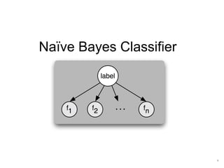
8. Naïve Bayes Classifier
Learning
1. Compute the class prior table which contains all P(c)
2. Compute the likelihood table which contains all P(xi|c) for all possible
combination of xi and c;
Scoring
1. Given a test instance X, compute the posterior probability of every class c;
2. Compare all P(c|X) and assign the instance x to the class c* which has the
maximum posterior probability
∏=
≈
K
i
i cPcXPXcP
1
)()|()|(
The constant term is ignored because it
won’t affect the comparison across different posterior
probabilities
∏=
=
N
i
iXPXP
1
)()(
∑=
+=
K
i
ic cXPcPc
1
*
))|(log())(log(maxarg
∑=
+≈
K
i
i cXPcPXcP
1
))|(log())(log()|(log
To avoid floating point underflow, we often need an optimization on the formula

9. Handling Insufficient Data
Problem
Both prior and conditional probabilities must be estimated from training data,
therefore subject to error. If we have only few training instances, then the
direct probability computation can give probabilities extreme values 0 or 1.
Example
Suppose we try to predict whether a patient has an allergy based on the
attribute whether he has cough. So we need to estimate P(allergy|cough). If
all patients in the training data have cough, then P(cough=true|allergy)=1 and
P(cough=false|allergy)=1-P(true|allergy)=0. Then we have
• What this mean is no not-coughing person can have an allergy, which is
not true.
• The error is caused by there is no observations in training data for non-
coughing patients
Solution
We need smooth the estimates of conditional probabilities to eliminate zeros.
0)()|()|( ==∝= allergyPallergyfalsecoughPfalsecoughallergyP

10. Laplace Smoothing
Assume binary attribute Xi, direct estimate:
Laplace estimate:
equivalent to prior observation of one example of class k where Xi=0 and one
where Xi=1
Generalized Laplace estimate:
• nc,i,v: number of examples in c where Xi=v
• nc: number of examples in c
• si: number of possible values for Xi
ic
vic
i
sn
n
cvXP
+
+
==
1
)|( ,,
2
1
)|0( 0,,
+
+
==
c
ic
i
n
n
cXP
2
1
)|1( 1,,
+
+
==
c
ic
i
n
n
cXP
c
ic
i
n
n
cXP 0,,
)|0( ==
c
ic
i
n
n
cXP 1,,
)|1( ==

11. Comments on Naïve Bayes Classifier
• It generally works well despite blanket independence assumption
• Experiments shows that it is quite competitive with other methods on
standard datasets
• Even when independence assumptions violated, and probability estimates
are inaccurate, the method may still find the maximum probability category
• Hypothesis constructed directly from parameter estimates derived from
training data, no search
• Hypothesis not guaranteed to fit the training data