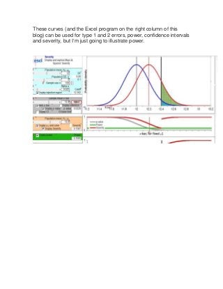
These curves (and the Excel program on the right column on the errorstatistics blog) can be used for type 1 and 2 errors, power, confidence intervals and severity, but I’m just going to illustrate power.

1. These curves (and the Excel program on the right column of this
blog) can be used for type 1 and 2 errors, power, confidence intervals
and severity, but I’m just going to illustrate power.

2. EXAMPLE SET 1: illustration using the Excel program
The curves in the Excel example depict the hypotheses in test T+, the
one-sided Normal test of
H0: μ ≤12 (blue curve) against H1: μ >12 (red curve).
Null (or test) hypothesis H0: X is Normal (µ, σ /√n), and µ = 12.
Alternative H1: X is Normal (µ, σ /√n), and µ >12.
Each hypothesis, being statistical, assigns probabilities to the
different values of X, and thus to the different values of the sample
mean X . Those are the heights of the curves. Areas under the curve
are probabilities for events like { X > 12.4}.
EXAMPLE SET 1: Throughout, keep σ = 2, and n = 100. So σ /√n =
2/10. Note: σ /√n is the standard deviation of X , I will sometimes
abbreviate this as σx because it’s too hard to get an x-bar as a
subscript of σ. (Ignore the lines under the curves for now, just look at
the curves and the boxes on the left.)
Let’s specify the test rule: the test T+ will reject H0 whenever X > 12 +
2 σ /√n
T+ reject H0 if and only if { X > 12.4}.
For { X < 12.4}. “do not reject” (i.e., accept) H0 .
{ X > 12.4}. is the rejection region of the test.
This test has a probability of rejecting H0 under the assumption we
are in the world of the first curve, i.e., assuming μ =12, of .023 (with a
slight approximation). This is the probability of a type 1 error, alpha.
(1) P[{ X > 12.4}; μ =12] = .023
In the picture, this is shown as the turquoise area under the curve. It
is also written as the 4th entry in the turquoise box on the left. The
turquoise box lists: the population mean (as given in the null of the
test, which we keep at 12) the population SD, σ, which we keep at 2,
the sample size, n, which (for Example Set 1) we keep at 100. Below
that is alpha, which we keep at .023 for this example set.

3. The only thing to be changed is the alternative (red) curve. The point
is to see the shifts in the probability test T+ rejects the null under
different assumptions for the alternative. Even though the alternative
is still H1: μ >12, we will compute the probability of rejection under
different point values μ1 greater than 12.
(2) P[{ X > 12.4}; μ = μ1] = The Power of test T+ (to reject H0) when
the true value of μ is μ1
We can abbreviate this as POW( μ1 ).
_______________________________________________________
The grey box on the left shows the sample mean X . For Example set
1, we will not change this. We assume X just makes it to the cut-off
for rejection, i.e., 12.4.
X = 12.4.
The gray box also shows the corresponding p-value which is ~.023
_______________________________________________________

4. Example 1.1
Finally we get to the good part. The figure below shows the case
where the alternative is μ = 12.2. That is, it sets μ1 = 12.2 in the
bottom, peachy-colored, box on the left.
We would like to know
(2a) P[{ X > 12.4}; μ = 12.2] = The probability test T+ would reject H0
when the true value of μ is 12.2.
POW( 12.2).
What is it? It is the green area under the red curve, which is .16. Why
do we look at the area under the red curve, rather than under the blue
curve? Because to the right of “;” in (2a) is μ = 12.2. It’s asking for a
calculation assuming we are in the hypothesized red world. So
imagine you’re in the red curve world where μ = 12.2: the probability
{ X > 12.4} is .16.

5. Example 1.2
Now consider the alternative μ = 12.3.
(2b) P[{ X > 12.4}; μ = 12.3] = The probability test T+ would reject H0
when the true value of μ is 12.3.
=.3
= POW( 12.3).

6. Example 1.3
Now consider the alternative μ = 12.4.
(2c) P[{ X > 12.4}; μ = 12.4] = The probability test T+ would reject H0
when the true value of μ is 12.4.
=.5
= POW( 12.4).

7. Example 1.4
Now consider the alternative μ = 12.5.
(2d) P[{ X > 12.4}; μ = 12.5] = .7
= POW( 12.5).