Research finding that the relation between the returns on investable commodity and U.S. equity indices has not changed significantly in the last fifteen years. Refutes the theory of a "market of one" where under stress all asset classes move together.

1. Commodities and Equities: A “Market of One”?
Bahattin Büyükşahin Michael S. Haigh Michel A. Robe1
June 9, 2008
Abstract
Amidst a sharp rise in commodity investing, many have asked whether
commodities nowadays move in sync with traditional financial assets. We
provide evidence that challenges this idea. Using dynamic correlation and
recursive cointegration techniques, we find that the relation between the
returns on investable commodity and U.S. equity indices has not changed
significantly in the last fifteen years. We also find no evidence of any
secular increase in co-movement between the returns on commodity and
equity investments during periods of extreme returns.
JEL Classification: G10, G13, L89
Keywords: Commodities, Equities, Dynamic conditional correlations, DCC,
Cointegration, Extreme-event returns.
1
Buyuksahin: U.S. Commodity Futures Trading Commission (CFTC), 1155 21st Street, NW, Washington,
DC 20581. Tel: (+1) 202-418-5123. Email: bbuyuksahin@cftc.gov. Haigh: Commodities Derivatives
Trading, Société Générale Corporate and Investment Banking, 1221 Avenue of the Americas, New York,
NY 10020. Tel: (+1) 212-278-5745. Email: michael.haigh@sgcib.com. Robe: CFTC and Department of
Finance, Kogod School of Business at American University, 4400 Massachusetts Avenue, NW,
Washington, DC 20016. Tel: (+1) 202-885-1880. Email: mrobe@american.edu. We thank the Editor, John
Doukas; our discussant at the 2008 EFMA Symposium on Risk and Asset Management in Nice, Joëlle
Miffre; as well as Celso Brunetti, Francesca Carrieri, Vihang Errunza, Pat Fishe, Andrei Kirilenko,
Delphine Lautier, Jim Moser, David Reiffen, Andy Smith, and workshop participants at the CFTC for
helpful comments and suggestions. All remaining errors and omissions, if any, are the authors' sole
responsibility. This paper reflects the opinions of its authors only, and not those of the CFTC, the
Commissioners, or any other staff upon the Commission.
1

2. ``As more money has chased (...) risky assets, correlations have risen. By the
same logic, at moments when investors become risk-averse and want to cut their
positions, these asset classes tend to fall together. The effect can be particularly dramatic
if the asset classes are small -- as in commodities. (...) This marching-in-step has been
described (...) as a 'market of one'." The Economist, March 8th, 2007.
1. Introduction
In the past decade, investors have sought an ever greater exposure to commodity
prices – by directly purchasing commodities, by taking outright positions in commodity
futures, or by acquiring stakes in exchange-traded commodity funds (ETFs) and in
commodity index funds. This pattern has accelerated in the last few years. To wit,
Standard and Poor's GSCI index was created by Goldman Sachs in 1991. This world-
production weighted index tracks the prices of major physical commodities for which
there are active, liquid futures markets. As recently as 1999, the sums invested in
investment vehicles tracking this index were estimated at less than 5 billion dollars.
Nowadays, however, investments linked to the GSCI or to one of five other prominent
commodity indices exceed 140 billion dollars. In a similar vein, the first-ever commodity
exchange traded fund (the streetTRACKS Gold Shares ETF) was started in November
2004. As of May 2008, its market capitalization exceeds 17 billion dollars, and it has
been joined by numerous commodity ETF competitors.
One naturally wonders whether this sharp increase in investor appetite for
commodities has had a significant impact on the pricing of related financial instruments.
One reason why it could have had an impact is if the large-scale arrival of financial
institutions in commodity markets has led to a reduced scope for cross-market arbitrage
opportunities (as in Basak and Croitoru, 2006) and, in the process, has more closely
linked commodity and equity markets. Another channel for tighter links between
commodity and equity markets is if financial institutions respond differently from
commercial traders to extreme stock market movements – in particular, if sharp
downward movements in one market force financial investors to liquidate positions in
commodity markets so as to raise cash for margin calls. In this paper, we investigate the
relation (or lack thereof) between ordinary as well as between extreme returns on passive
investments in commodity and equity markets.
Because much of the new commodity exposure has been achieved through direct
or indirect participation in futures markets, it should be reflected in the magnitude and
composition of commodity futures trading. Haigh, Harris, Overdahl, and Robe (2007;
henceforth, HHOR) confirm this intuition, using proprietary data on trader positions in
the world's largest-volume futures contract on a physical commodity – the New York
Mercantile Exchange's WTI sweet crude oil futures. HHOR show that greater market
participation by commodity swap dealers and hedge funds has been accompanied by a
change in the relation between crude oil futures prices at different maturities and greater
price efficiency. Specifically, the prices of one-year and two-year futures have become
cointegrated with the price of near-month futures, for the first time ever, since mid-2004.
Whereas this previous research documents that the prices of different-maturity
commodity futures have recently become much more closely linked, we use dynamic
2

3. correlation and recursive cointegration techniques to show that the degree of co-
movement between benchmark commodity- and equity-investment returns has not
changed materially over the course of the last fifteen years. In particular, notwithstanding
the surge in commodity investment flows, the already very low correlation between the
rates of return on passive investments in these two asset classes has become negative in
the last five years. Our results are similar in spirit to the finding that, despite increased
capital flows to emerging markets in the years following their financial liberalization and
despite greater integration with world equity markets, cross-market return correlations
did not increase enough to diminish the benefit, to U.S. investors, of diversifying into
emerging-market stocks (Bekaert and Harvey, 2000; Carrieri, Errunza and Hogan, 2007).
We use Standard and Poor's S&P 500 return and GSCI total return data to proxy
for the rates of return on representative unlevered investments in, respectively, U.S.
equities and commodities (we obtain qualitatively similar results with two other widely-
used indices: Dow Jones' DJIA equity and DJ-AIG total return commodity indices2).
Since much of the commodity investment boom is still quite new, any change in pricing
relationships is likely to be a recent phenomenon. HHOR, for example, do not find
pricing efficiency changes across crude oil futures maturities until September 2003 (for
one-year contracts) or May 2004 (for both one- and two-year contracts). It is therefore
important to utilize recent data. Accordingly, we use daily, weekly and monthly returns
from January 1991 (when GSCI products first became available) through May 2008.
To identify possible changes in the co-movements between the asset return series,
we run all of our analyses on the entire sample period and then focus in particular on
three successive sub-periods: June 1992 to May 1997; June 1997 to May 2003; and, June
2003 to June 2008. The first sub-period predates the commodity investment boom, while
the third sub-period covers the interval of time during which financial traders greatly
increased their participation in commodity futures markets (HHOR). These two sub-
periods correspond to times of economic expansion. The second sub-period, in contrast,
includes an economic contraction as defined by the National Bureau of Economic
Research (NBER). More importantly, June 1997 to May 2003 captures the Asian crisis;
the Russian and Argentinian sovereign defaults; and, the U.S. stock-market bubble and its
direct aftermath. By choosing these specific sub-periods, we can thus establish that our
results are not driven by the relation between commodities and equities (or the relation
between their volatilities) during times of stock-market or macro-economic turbulence.
We find statistically significant differences in the means and standard deviations
of the rates of returns across the two asset classes and, for each asset class, across the
three sub-periods. By contrast, we find only small differences in cross-asset correlations
for the three sub-periods: the simple correlation between equities and commodities, which
was slightly positive between 1992 and 1997, is slightly negative between 2003 and
2008. We obtain qualitatively similar results at all return frequencies.
2
Unlike the GSCI, which uses weights that reflect world-production figures and is consequently heavily
tilted toward energy commodities, the DJ-AIG commodity index is specifically designed to provide a
“diversified benchmark for the commodity futures market.” In particular, it assigns a weight of only about
30% to energy commodities, including about 13% to crude oil. By comparison, as of mid-July, 2007, the
GSCI assigned a weight of more than 70% to energy commodities, including 36% to crude oil (WTI nearby
contract). Other GSCI competitors include the Deutsche Bank Liquid Commodity Index, Rogers
International Commodity Index, and Reuters-CRB.
3

4. Notwithstanding the fact that the simple cross-correlations are almost zero in all
three sub-periods, we find that rolling measures of the correlations between equity and
commodity return series fluctuate substantially throughout the sample period. The pattern
of fluctuations, however, does not appear to change during the entire sample period. We
confirm these analyses using the dynamic conditional correlation (DCC) methodology
proposed by Engle (2002). The range of values taken by DCC estimates is indeed quite
wide: weekly values, for example, can be as low as − 0.5 or as high as + 0.5 . Most of
the time, however, the DCC estimates are close to 0. What is more important, we find no
evidence of a secular increase in correlations in the last few years.
Correlation estimates are relevant for short-term investors. For long-term
investors, however, the key issue is whether there exists a long-term relation between the
prices of commodity and equity investment even though these prices may diverge in the
short term (Kasa, 1992). To answer this question, we apply recursive cointegration
techniques (Johansen, 1998, 1991; Johansen and Juselius, 1990) to examine the stability
and the possible strengthening over time of the relation between equity- and commodity-
investment price series. This analysis complements our other results: except for a short
period in the late 1990's, we find little statistical evidence of cointegration – and none in
the last eight years. The implication is that passive investors can still achieve substantial
gains by diversifying portfolios across the two asset classes.
Although there is no evidence of a structural shift in correlation and cointegration
levels, it could still be the case that financial and commodity markets have become a
“market of one” during extreme events. Hartmann, Straetmans and de Vries (2004), for
example, find evidence of cross-asset extreme linkages in the case of bond and equity
returns from the G-5 countries. Using a different approach, Longin and Solnik (2001)
provide evidence that international equity-market correlations increase in bear markets.
Here, we first identify the days and weeks during which returns on equity indices
were at least one or two standard deviations away from their means, and then analyze the
contemporaneous returns on investable commodity indices. Contrary to extant findings
on extreme linkages between other asset markets, this first analysis finds little relation
between exceptionally large returns on equities and those on commodities. This is true
for the whole sample period as well as for all three of our sub-periods; for positive as
well as for negative exceptional returns; and, for periods of stock market upturns as well
as downturns. We then use a technique similar to Longin and Solnik’s (2001) to analyze
equity-commodity linkages when the returns on equity and commodity indices both take
values in the tails of their respective distributions. We only find weak extreme-event
correlations are. Interestingly, whereas Longin and Solnik find high positive correlations
across international equity markets in down markets, we document that the equity-
commodity correlation is mildly positive in the upper tail but is negative in the lower tail.
That is, conditional on both equity and commodity returns being very poor, the two return
series are negatively correlated. This finding highlights yet another aspect of the diversi-
fication benefits that commodities provided to equity investors between 1991 and 2008.
In sum, the lack of greater return co-movement across equities and commodities
suggests that commodities have retained their role as a portfolio diversification tool. The
import of this conclusion cannot be overstated, since many academics and practitioners
have long called for substantial allocations to commodities as an asset class for the
4

5. purposes of return generation and portfolio diversification.3
The remainder of the paper proceeds as follows. Section 2 describes the data.
Section 3 presents the correlation analyses. Section 4 shows the robustness of our results
to alternative methodological choices. Section 5 concludes.
2. Data and descriptive statistics
This section discusses the data and gives summary statistics for the return series.
2.1 Returns data
We take the perspective of a passive investor on the relation between
commodities and traditional financial investments. Modern portfolio theory suggests that
the relevant information matrix for such an investor includes the expected asset returns,
the variances of these returns, as well as cross-asset correlations.
To assess short-term correlations, we use daily, weekly, and monthly returns and
return volatilities on four commodity and equity indices that are widely used to construct
portfolios.4 We focus on results for weekly (Tuesday to Tuesday) holding-period returns,
and provide a brief discussion of our (qualitatively similar) findings for daily and
monthly returns. To analyze long-term cointegration, we use the Tuesday close prices for
the same four indices.
For equities, we use Standard and Poor's S&P 500 index; in robustness checks, we
use Dow-Jones's DJIA index.5 For commodities, we focus on the unlevered total return
on Standard and Poor's S&P GSCI (formerly, the Goldman Sachs Commodity Index),
i.e., the return on a “fully collateralized commodity futures investment that is rolled
forward from the fifth to the ninth business day of each month.” While the GSCI
includes twenty-four nearby commodity futures contracts, it is heavily weighted toward
energy. For robustness checks, we use total (unlevered) returns on the second most
3
See, e.g., Ankrim and Hensel (1993), Froot (1995), Huberman (1995), and Satyanarayan and Varangis
(1996) for early work on how commodities help reduce an investor's unconditional portfolio risk. See also
Erb and Harvey (2006), Gorton and Rouwenhorst (2006), and Miffre and Rallis (2007) for evidence on the
strategic and tactical values of commodity investments. The data series in these newer papers end in 2004
and, hence, do not cover the period during which took place much of the growth in financial traders’
positions in commodity futures markets.
4
We measure the percentage rate of return on the Ith investable index in period t as rIt = 100 Log(PIt / PIt-1),
where PIt is the value of index I at time t. We measure the volatility of an index in period t as (rIt - ā)2,
where ā is the mean value of rIt over the relevant sample (sub-)period.
5
We use returns on both of these equity indices that are exclusive of dividend yields. This approach leads
to an underestimation of the expected returns on equity investments (Shoven and Sialm, 2000). However,
insofar as large U.S. corporations smooth dividend payments over time (Allen and Michaely, 2002), the
correlation estimates that are the focus of our paper should be essentially unaffected.
5

6. widely used investable benchmark, Dow-Jones's DJ-AIG total-return commodity index
(henceforth, DJ-AIG). This rolling index, which is composed of futures contracts on
nineteen physical commodities, was designed to provide a “diversified benchmark for the
commodity futures market.”
We also analyze potential changes in the relation between the rates of returns on
specific types of commodities. For this purpose, we use daily, weekly, and monthly total
returns on several investable sub-indices representing key components of the GSCI:
Energy, Non-Energy, Industrial Metals, Precious Metals, Agriculture, and Livestock.
We obtain the price data for all four indices (GSCI, DJ-AIG, S&P 500 and DJIA)
and the GSCI commodity sub-indices from Bloomberg. Our data cover more than
seventeen years, from January 2 1991 through May 2008. We also provide results for
three successive sub-periods: June 1, 1992 to May 31, 1997; June 1, 1997 to May 31,
2002; and, June 1, 2003 to May 26, 2008.
2.2 Returns on Equity and Commodity Indices: Summary Statistics
Table 1 presents some descriptive statistics, for the entire sample period, for the
two equity- and the two commodity-return series. Panels 1, 2 and 3 present statistics for,
respectively, daily, weekly and monthly returns.6
From January 1991 through mid-2008, the mean weekly total rate of return on the
GSCI was 0.16% (or 8.43% in annualized terms), with a minimum of -14.59% and a
maximum of 7.78%. The typical rate of return varies sharply across the sample period: it
averaged 0.14% in 1992-1997 (7.45 % annualized); 0.045% in 1997-2003 (or a mere
2.36% annualized); and, jumped to 0.35% in 2002-2007 (19.79% annualized). The
corresponding figures are very similar for the DJAIG total return index – with two
exceptions. One exception is the first sub-period (1992-1997), when the average weekly
return was 0.205% for the DJAIG versus 0.138% for the GSCI; Figure 1, which plots the
levels of the four indices, indeed shows that the GSCI did not start appreciating until the
end of 1996 whereas the DJAIG started appreciating in 1994. The second exception is in
the third sub-period, when the DJAIG yielded 0.29% per week on average, vs. 0.35% on
average for the GSCI. Figure 1 shows that, while the two indices did grow in sync during
much of that period (except in the second half of 2006), the GSCI indeed grew more.
During the entire sample period, the mean weekly rate of return on the S&P 500
was only slightly higher than that on commodities: 0.17% (or 8.99% in annualized
terms), with a minimum of -12.17% and a maximum of 12.37%. While the lowest weekly
rate of return on all four indices is found in the second sub-period, the median weekly
rate of return on the commodity indices was very low (0.023% on the GSCI and 0.014%
on the DJAIG) between June 1997 and May 2003, whereas the S&P 500 equity index had
its highest median weekly rate of return during the same period (+0.37%). In a similar
vein, whereas the highest equity returns took place in the first sub-period, the peak for
commodities is observed in the third sub-period. These observations suggest that equities
and commodities do not move together.
6
For weekly returns, tables presenting the corresponding statistics for each of the three successive sub-
periods are available from the authors upon request.
6

7. Consistent with the fact that the DJAIG is by construction more diversified than is
the GSCI, the standard deviation of the weekly rates of return is much lower for the DJ-
AIG (1.80% for the whole sample) than for the GSCI (2.68%). This pattern of
approximately 45% greater GSCI volatility is observed in all three sub-periods: 1.81% vs.
1.26% in 1992-1997; 2.87% vs. 1.88% in 1997-2003; and, 3.17% vs. 2.20% in 2003-
2008. Standard deviations increase throughout the sample for commodities, while they
peak in the second sub-period for equities.
Panels E and F show similar patterns for daily and monthly returns that Panels A
to D showed for weekly returns, i.e.:
• Between 1991 and 2008, the rates of return on commodity indices were
similar to those on equity indices. However, the rank-ordering of returns on
these two asset classes fluctuates dramatically over the course of the sample
period. For example, equity returns trounce commodity returns in 1992-1997,
but commodity returns are approximately double equity returns in 2003-2008.
• The rates of return on equites are somewhat more volatile than those on a
well-diversified basket of commodities (represented by the DJAIG), except in
the last five years (2003-2008).
• The rates of return on the GSCI are the most volatile throughout the entire
sample period. Of note, the GSCI returns are approximately 40-50% more
volatile than those on the DJAIG.
2.3 Simple Cross-Asset Correlations: Returns and Return Volatilities
Figure 1 gives some preliminary insights into the co-movements between the
commodity and equity indices. This graph allows the reader to visualize which sub-
periods help determine the co-movements between the index returns that are summarized
by the return correlations presented in Table 2. In particular, it suggests a high correlation
between the two equity indices; a positive, but somewhat weaker, correlation between the
two commodity indices; and, a weak or possibly negative correlation between the equity
and commodity indices, especially during the second sub-period (June 1997 - May 2003).
Table 2 quantifies these first impressions by providing an overview of the simple
correlations between the two four benchmark asset-return series. This summary table is
helpful for the interpretation of the empirical results in Section 3. Panels 1, 2 and 3 of
Table 2 are for, respectively, daily, weekly and monthly returns. For weekly returns,
Tables 2B, 2C and 2D present the corresponding statistics for each of the three successive
five-year sub-periods.
As one would expect, the simple correlation between the returns on the DJIA and
S&P 500 equity indices is very high (more than 0.93 from 1991 to 2008), especially in
the last five years (0.96). Likewise, the rates of return on the two commodity indices are
strongly positively correlated. At all three return frequencies, their simple correlation is
about 0.89 for the whole sample; it is strongest in the second sub-period (0.93) and is
slightly weaker in 1992-1997 at the weekly return frequency.
In sharp contrast, equity-commodity cross-correlations are typically very low or
even negative:
7

8. • In the case of daily returns, Panel 1 shows that the rates of return on the
commodity indices exhibit very little correlation with either of the equity
returns, with the coefficient estimates ranging from -0.0615 to 0.0014
depending on the index pair and the time period.
• For weekly returns, Tables 2B and 2C show that the “highest” weekly
correlations, a mere 0.09 to 0.13 depending on the index, were observed in the
first (1992-1997) and second (1997-2003) sub-periods.
• For monthly returns, equity-commodity correlations are not statistically
significantly different from zero for the entire sample period.7
In short, despite a commonly-expressed view that both equity and commodity
prices have increased in tandem since 2003, the correlation between commodity and
equity returns is almost zero in our third sub-period – indeed, the total returns on the
GSCI are negatively correlated with the returns on both equity indices during that period.
Figure 1 suggests that, to the extent that the correlations were at all positive prior to 2002,
the likely reasons are joint run-ups in commodity and equity prices in 1995-1997 and
again in the eighteen month period from late 1998 through Spring 2000.
One clear conclusion from Table 2 is that the simple correlation between the rates
of return on commodities and equities are typically not statistically significantly different
from zero. Even if there is little correlation between the first moments of the return series,
though, it may still be the case that the second moments of the returns are related. Table
3 shows the correlation between return volatilities, at the weekly frequency, for the full
sample period (Panel A) and our three sub-periods (Panels B, C and D). Similar to the
evidence in Table 2 regarding return correlations, return-volatility correlations are always
extremely close to zero. In the last five years of the data series, likewise, correlations
between equity and commodity return volatilities are even slightly negative (though not
statistically significantly different from zero).
2.4 Returns on Specific Categories of Commodities
2.4.1 Summary Statistics
Table 4 provides summary statistics for the unlevered (total) rates of return on six
investable sub-indices representing key components of the S&P GSCI index: the GSCI
Energy, Non-Energy, Industrial Metals, Precious Metals, Agriculture, and Livestock
investable indices. We focus on Panel 2 (weekly returns) for the sake of brevity, because
the results are similar for daily and monthly return series (Panels 1 and 3, respectively).
Over the entire sample period, individuals who invested in Energy or Metal sub-
indices experienced greater average returns (but also more volatility) than investors in
7
At the monthly frequencey, the GSCI's correlation with the S&P 500 and the DJIA was 0.27 in 1992-1997
(statistically significantly positive at the 5% level); this correlation became statistically significantly
negative in 2002-2007 (-0.25 with the DJIA and -0.3 with the S&P 500). Tables for sub-periods and sub-
indices are available from the authors upon request.
8

9. other commodity sub-indices. However, performance rankings vary significantly from
period to period. Industrial as well as Precious Metals, for example, both underperform
all other commodity sub-indices between 1992 and 1997, but beat all but Energy between
2003 and 2008. In a similar vein, Agriculture outperforms all other sub-indices in 1992-
1997 but is the worst performer in 2003-2008.
2.4.2 Simple Correlations
Table 5 shows the simple correlations between the unlevered rates of return on the
S&P 500 equity index, the S&P GSCI, and the six narrow commodity benchmarks
introduced in Table 4. Again, Table 5 focuses on weekly returns. Table 5A presents
statistics for the entire sample period, while Tables 5B, 5C and 5D present the
corresponding statistics for each of our three successive sub-periods. Four patterns
emerge from Table 5:
• Equity returns exhibit very little correlation with the returns on any of the
commodity sub-indices. The highest weekly individual correlation is for
Industrial Metals, but even that figure is a mere 0.13 over the whole sample
(Table 5A), peaking at 0.20 in 2003-2008 (Table 5D). All the other cross-
correlations are less than 0.17, and quite a few are slightly negative.
• There is no evidence of a material increase, over time, of the correlation
between the returns on equities and those on either the Agriculture or the
Livestock sub-indices.
• Consistent with the fact that the GSCI is a value-weighted index and is
consequently heavily weighted toward energy (as energy contracts make up
the world's largest commodity futures markets), the unlevered returns on the
GSCI and on the Energy sub-index are very highly positively correlated –
between 0.94 and 0.98 depending on the sample period. In contrast, the
correlation between the returns on the entire GSCI index and those on the
Non-Energy sub-index range from 0.39 to 0.43 depending on the sub-period.
• The returns on the Non-Energy sub-index are strongly positively correlated
with the returns on all the other GSCI sub-indices (but not with the Energy
sub-index). This finding suggests the possibility of a common economic
variable driving the returns on most types of commodities.
In addition to the return correlations between equity and commodity sub-indices,
a relevant piece of information for some investors is the correlation between the return
volatilities of those assets. The numbers in Column 1 in Table 6 show these return-
volatility correlations, from 1991 to 2008. These numbers strengthen our conclusion that
the correlation between the volatilities of equities and commodities are always very low
and almost never statistically significantly different from zero. Indeed, Table 6 shows
that the correlations between return volatilities are if anything even lower than the
correlation between the returns themselves.
9

10. 3. Short-Term Co-Movements
Tables 1B, 1C and 1D, and Tables 3B, 3C and 3D, in the Appendix show that the
unconditional return volatilities, as measured by the standard deviations of returns, vary a
lot over time. In particular, the weekly rates of return on equities were 50% more volatile
in the third sub-period (2003-2008) than in the first (1992-1997). Even more strikingly,
the standard deviation of the returns on commodity investments almost doubled over the
course of our entire sample period.
In contrast, although the unconditional correlations between the rates of returns on
equity and commodity investments vary somewhat from sub-period to sub-period, Tables
2B, 2C and 2D suggest that these fluctuations are quite mild and that the correlations are
always close to zero. Put differently, the analysis in Section 2 seemed to suggest that
commodity returns exhibit consistently low correlations with their equity counterparts.
Before concluding that commodities provide a good hedge for equity portfolios,
however, one should account for possible time variations in these correlation measures.
In this Section, we provide estimates of the intensity of co-movements (or the lack
thereof) that account for time variations in the various moments of the return series.
3.1 Methodology
Measuring the relationship between variables at various points in time, rather than
using a single correlation coefficient over the entire sample period, provides information
on the evolution of the relationship over time. For this purpose, simple correlation
measures such as rolling historical correlations and exponential smoothing are widely
used in the literature.
Rolling historical correlations take into account the time-varying nature of the re-
lationship between variables straightforwardly, by calculating the correlation at any point
in time as the estimate for a specified window (say, k observations) that does not overlap
with the full sample. The correlation is first estimated over sub-periods 1 to k , then over
sub-periods 2 to k + 1 , and so on. The rolling historical correlation estimator is thus:
t
∑x x
1, s 2, s
ρ12,t +1 =
ˆ s =t − k
(1)
⎛ t 2 ⎞⎛ t 2 ⎞
⎜ ∑ x1, s ⎟⎜ ∑ x2, s ⎟
⎝ s =t − k ⎠⎝ s =t − k ⎠
where x1 and x2 are the deviations from the means of the two random variables of
interest, with mean zero.
Although this simple estimation technique provides some information on the
evolution of relationship between two variables, it suffers from assigning an equal weight
to all observation in the estimation window and zero weight to older observations. It also
raises the issue of window-length determination. On the one hand, if the window is too
narrow, one runs the risk of ignoring important observations in the data by giving zero
10

11. weight to these observations. On the other hand, if the window is too wide, old
observations will be given weight even though they may not be relevant to the analysis.
To overcome these problems, exponential smoothing techniques assign declining
weights to older observations based on a parameter, λ , without any prior determination
on the amount of past data to be used in the analysis. The exponential-smoothing
estimator can be written as
t
∑λ t −s
x1, s x2, s
ρ12,t +1 =
ˆ s =1
(2)
⎛ t t − s 2 ⎞⎛ t t − s 2 ⎞
⎜ ∑λ x1, s ⎟⎜ ∑λ x2, s ⎟
⎝ s =1 ⎠⎝ s =1 ⎠
One drawback of this second approach is that the user must adopt an ad hoc
approach to choose smoothing parameter λ . Engle (2002) used λ = 0.94 to analyze daily
returns on the major equity indices. We use the same value for monthly and weekly
returns, but set λ = 0.97 for daily returns.
More importantly, like the rolling historical correlation, the exponential-
smoothing technique cannot adequately account for changes in volatility. The sensitivity
of the estimated correlation to volatility changes restricts inferences about the true nature
of the relationship between variables. Since the estimated correlations are subject to
volatility shocks, interpreting these correlations becomes more difficult especially during
high volatility periods.
The Dynamic Conditional Correlation methodology (DCC) developed by Engle
(2002) helps to remedy this problem. The DCC model is based on a two-steps approach
to estimating the time-varying correlation between two series. In the first step, time-
varying variances are estimated using a GARCH model. In the second step, a time-
varying correlation matrix is estimated using the standardized residuals from the first-
stage estimation.
More formally, consider a n × 1 vector of normally-distributed with mean zero
and covariance matrix H t returns series rt of n assets are assumed the have the
following structure:
rt ~ N (0, H t ) (3)
H t = Dt Rt Dt (4)
where, H t is the conditional covariance matrix; Rt is the time varying correlation matrix;
and, Dt is a diagonal matrix of time-varying standard deviations given by
Dt = diag Et −1 (ri 2t ) = diag hi ,t . The hi,t can be thought of as univariate GARCH
,
models, so the standardized disturbance can be expressed as ε i ,t = ri ,t / hi ,t = Dt−1 ri ,t ,
where ε i ,t ~ N (0, Rt ). Consider the following conditional correlations:
Et −1 [ri ,t r j ,t ]
ρ ij ,t = (5)
Et −1 [ri 2t r j2,t ]
,
11

12. Re-writing these conditional correlation in terms of standardized residuals from
GARCH estimates yields:
ρ ij ,t = Et −1ε i ,t ε j ,t (6)
This implies the equivalence of conditional correlation of returns and conditional
covariance between the standardized disturbances. Therefore, the matrix R represent the
time-varying conditional correlation matrix of returns as well as the conditional
covariance matrix of the standardized residuals (Engle ,2002).
The DCC model of Engle (2002) suggest the following dynamics of the
correlation matrix:
-1 −1
Rt = Qt* Qt Qt* (7)
Qt = (1 − α − β )Q + α (ε i ,t −1ε j ,t −1 ) + β Qt −1 (8)
where Q is the unconditional correlation matrix of standardized residuals and Q*t is a
diagonal matrix composed of square root of the diagonal elements of Qt. The correlation
estimator is given by the typical element of Rt in the form of
qij ,t
ρ ij ,t =
qii ,t q jj ,t
This specification ensures the mean reversion as long as α + β < 1 . The resulting
estimator is called DCC by loglikelihood with mean reverting model. The log-likelihood
of the DCC model outlined above is given by :
1 T
L=− ∑(n log(2π ) + 2 log(| Dt |) + log(| Rt |) + ε ' RT−1ε )
2 t =1
In essence, the log-likelihood function has two components: the volatility part,
which contains terms in Dt ; and the correlation part, which contains terms in Rt . In the
first stage of the estimation, n univariate GARCH(1,1) estimates are obtained, which
produces consistent estimates of time-varying variances ( Dt ). In the second stage, the
correlation part of the log-likelihood function is maximized, conditional on the estimated
Dt from the first stage.
We use rolling historical correlation, exponential smoother, and dynamic
conditional correlation by log-likelihood for mean-reverting model estimation to analyze
the dynamic properties of the relevant variables.
3.2 Equities and Commodities
Figures 2 to 5 plot the estimates of the time-varying correlation between the
unlevered rates of return on investable equity and commodity indices over the sample
period. Figure 2, 3, 4, and 5 provide information on the correlations between,
12

13. respectively, the S&P 500 and GSCI; S&P 500 and DJ-AIG; DJIA and GSCI; and, DJIA
and DJ-AIG. Figure 6 provides similar plots for the correlation between the two equity
indices (S&P 500 and DJIA). Note that, in Figures 2 and 3, three panels are provided:
Figures 2A and 3A are for weekly returns; Figures 2B and 3B, for daily returns; and
Figures 2C and 3C, for monthly returns.
For weekly returns, each panel or Figure contains three plots, one for each of the
estimation methods outlined above: rolling historical correlation; exponential smoother
with smoothing parameter 0.94; and dynamic conditional correlation (DCC) by log-
likelihood for mean-reverting process. For the sake of brevity, only the DCC estimates
are presented in the case of daily and monthly returns. The straight line running through
each graph shows the relevant simple correlation from Table 2, which is not an average
of any of the four time-varying correlation estimates. Several facts are immediately
apparent from these graphs.
• The correlation between equity and commodity returns fluctuates notably over
time. This finding holds regardless of the choice of equity or commodity
indices, in that the correlation time-patterns are the same for all four pairs of
investable indices.
• There is little evidence that correlations are any higher after 2002 than they
were prior to 2003. If anything, consistent with the results obtained with
simple correlations (see Table 2, in particular Table 2D), the time-varying
correlation graphs show that correlations are lower since 2003 than before.
• Notwithstanding some amount of fluctuation over time, the correlations
between equities and commodities are not often greater than 0.3. In contrast,
Figure 6 shows that the correlation between the two equity indices is very
high, typically well above 0.9.
In sum, equity-commodity return pairwise correlations fluctuate over the sample
period. Quite often, the correlation estimates are even negative. These findings underline
the importance of accurate measures of co-movement between asset returns necessary for
portfolio optimization.
3.3 Commodity Sub-Indices
Figures 7 and 8 complement the analysis of the previous subsection, by plotting
estimates of the time-varying correlations between the unlevered rates of return on
benchmark equity indices and on specific categories of investable commodity indices.
Figure 7 focuses on the difference between "Energy" and "Non-Energy" commodity
baskets. Figure 8 refines Figure 7 by breaking down the Non-Energy index further into
several investable sub-indices: Precious Metals, Industrial Metals, Agriculture, and
Livestock. All of the plots in Figures 7 and 8 are directly comparable, in that they are all
drawn using dynamic conditional correlations estimated by log-likelihood for mean-
reverting model. Figures 7 and 8 highlight four facts:
13

14. • There is a substantial amount of time variation in the correlations between
returns on equities and on both the Energy and Non-Energy commodity sub-
indices. Depending on the time sub-period, these correlations fluctuate
between -0.4 and 0.45. By contrast, the unconditional correlations are close to
zero across the entire sample period.
• Both the GS and DJ Energy sub-indices present pattrns of correlation with
equity indices that are extremely close to the corresponding patterns for the
comprehensive GSCI and DJ-AIG indices.
• Figure 8 suggests, however, that indices based on more narrow categories of
commodities exhibit less correlation with equities than the overall non-energy
index – suggesting possible diversification opportunities.8
• Finally, and importantly for the purpose of the present paper, it is readily
apparent from both Figures 7 and 8 that there is no obvious secular pattern
toward an increase in correlations in the last few years.
4. Long-term Co-Movements
The foregoing analysis indicates that the correlations between the equity and
commodity return series may have fallen amidst the commodity investment boom. The
very fact that these correlation estimates fluctuate significantly over time, however, is
evidence of their short-term nature. If there is a reason to suspect that equity and
commodity return should move together in the long run, however, a complementary
technique is required.
4.1 Cointegration Analysis
A large volume of research evaluates the degree of interconnectivity between
prices from different markets by employing time-series techniques that are appropriate
for non-stationary and co-integrated data. In particular, much work on applied co-
integration analysis has relied on Johansen’s multivariate approach (Johansen, 1988,
1991; Johansen and Juselius, 1990).
Johansen (1988) proposes and implements a unified vector autoregressive system
approach for testing cointegration. Johansen derived the maximum likelihood estimator
of the space of cointegration vectors and the likelihood ratio test of the hypothesis that it
has a given number of dimensions. The procedure involves the following stages:
• Model checking, determination of lag length;
• Determination of cointegration rank, trace and maximum eigenvalue statistic;
• Estimation of the cointegration space;
8
See Chong and Miffre (2008) and references cited therein for discussions of diversification strategies
using individual commodity futures.
14

15. The first step of the model building involves the choice of lag order. The most
common procedure is to estimate a vector autoregression using the undifferenced data.
Then we can use different information criteria to select the number of lag lengths. In our
analysis, we use Schwarz (SC) criteria to determine the optimal lag – 2 in our case.
After selecting the lag length, the Johansen procedure estimates a vector error
correction model (VECM) to determine the number of cointegrating vectors. According
to Johansen (1988), a general polynomial distributed lag process, xt , involving up to k
lags, can be written as:
xt = Π 1 xt −1 + ... + Π k xt −k + u t (9)
where xt is a vector of n variables of interest, Π i is an (n × n) matrix of parameters, and
u is n -dimensional Gaussian independently distributed random variables with zero mean
and variance matrix ( Λ ).This equation can be reformulated into VECM form:
Δxt = Γ1 Δxt −1 + ... + Γk −1 Δxt −k +1 + Θxt − k + u t (10)
where Γi = −Σ kj =i +1Π j , ( i = 1,2,..., k − 1 ), and Θ = Σ ik=1 (Π i − I ) . This way of specifying the
system contains information on both the short and long run adjustments to changes in xt ,
via the estimates of Γ and Θ , respectively. Assuming that x is I (1) , while r linear
ˆ
i
ˆ
t
combinations of xt are stationary, we can write
Θ = αβ ′, (11)
where α is the vector of adjustment coefficients; β is the cointegrating vector; and both
are ( n × r ) matrices. The approach of Johansen is based on the estimation of system (10)
by maximum likelihood, while imposing the restriction in (11) for a given value of r .
Johansen (1988) demonstrates that β can be estimated by regressing ΔX t and
X t − k on the lagged differences.
The next step in the Johansen approach involves testing the hypothesis about the
rank of the long run matrix Θ , or equivalently the number of columns in β . The
likelihood ratio test for the determination of the rank r is discussed in Johansen (1992).
In general, tests of the hypothesis that r ≤ q use the likelihood ratio test statistics:
λtrace (q ) = −TΣ kj = q +1log (1 − λ j )
ˆ (12)
This test is called the trace test. It checks whether the smallest k − q eigenvalues
are significantly different from zero. Furthermore, we can test H 0 : r ≤ q versus the more
restrictive alternative H 1 : r = q + 1 using
λmax (q) = −Tlog (1 − λq +1 )
ˆ (13)
15

16. This alternative test is the so-called maximum eigenvalue test, as it is based on the
estimated (q+1)th largest eigenvalue.
Most of the existing Monte Carlo studies on the Johansen methodology point out
that dimension of the data series for a given sample size may pose particular problems
since the number of parameters of the underlying VAR models grows very large as the
dimension increases. Likewise, difficulties often arise, when a given lag length of the
system is either over or under parameterized. Reimers (1992) argues that for small
samples, the Johansen procedure over-rejects when the null is true. To correct this bias,
he suggests an adjustment in the degrees of freedom in the trace statistics and the
maximum eigenvalue test statistics by replacing T by T − nk for small samples. The
corresponding degrees of freedom adjusted trace and maximum eigenvalue test statistics
can be written as:
λtrace (q ) = −(T − nk )Σ kj = q +1log (1 − λ j )
a ˆ
λa (q) = −Tlog (1 − λq +1 )
max
ˆ
We first perform a univariate Augmented Dickey Fuller unit root test to determine
the order of integration for each variable. Both variables (S&P GSCI total return index
and S&P 500 index) appear to be integrated of order one; that is to say, our variables are
nonstationary and they only become stationary after we take first differences. This
finding suggests that we cannot rely on standard regression procedures, since OLS
estimators have sampling distributions that are very different from those derived under
the assumption of stationarity. Therefore, we proceed with the Johansen cointegration
approach to determine whether there exists a long run relationship between our variables.
Table 7 shows the cointegration rank between S&P’s 500 and GSCI indices for the full
sample period. Trace statistics suggest the absence of any cointegrating vector between
commodity and equity indices. This result is consistent with the low-correlation that we
observe from our dynamic conditional correlation estimation.
4.2 Recursive Cointegration Analysis
To obtain an understanding of the dynamics of the relationship, which the
foregoing analysis cannot provide, we examine the dynamics and extent of relationship, if
any, between our indices using recursive cointegration method outlined in Hansen and
Johansen (1993). Recursive cointegration techniques allow us to test for the level of co-
integration among indices during our sample period. The recursive technique allows us
to recover two ECM representations. In the “Z-representation,” all the parameters of the
ECM ( β and α ) are re-estimated during the recursions, while under the “R-
representation” the short-run parameters ( α ) are kept fixed to their full sample values
and only the long run parameters ( β ) are re-estimated.
The logic behind the recursive cointegration technique is similar to Johansen’s
(1988) multivariate cointegration approach. Instead of using all observations, we start
with an initial sample period from t0 to tj to perform Johansen (1988) cointegration
16

17. approach and calculate the corresponding trace statistics for this sub-sample. Then, we
increase the sample size by 1 from t0 to tj+1 and calculate the relevant trace statistics for
this sample period. This process continues until we exhaust all the observations and, in
the final stage, we perform the cointegration analysis for the full sample and calculate the
trace statistics. Of course, the trace statistic calculated in the final stage is equal to
standard static trace statistics calculated with the Johansen (1998) method. The recursive
method, however, allows us to see the dynamics of the trace statistic.
We start with 52 weeks of observations and add one more week in each step until
we exhaust all our observations.9 We re-scale our trace statistics by the 95% quantile of the
trace distribution derived for the selected model without exogenous variables or dummies.
Re-scaled trace statistics suggest the rejection of null hypothesis of no cointegration if it is
above 1. In addition, to see whether there exist a cointegrating vector among our variables,
the slope of re-scaled trace statistic determines the direction of co-movements between our
variables. An upward slope indicates rising co-movement, while a downward slope for the
trace statistics reveals declining co-movement between our variables.
Figure 9 shows the R-1 form of the trace statistic, recursively calculated and
scaled by the 5% critical value. The dark blue line gives the estimate calculated using
data from the whole sample (i.e., from January 1991 through May 2008).10 Although
there is a large variation in trace statistics during our sample period, we can divide our
sample period into three distinctive periods.
• The first period, from January 1992 to May 1997, is characterized by a relatively
stable trace statistics that is generally below the threshold level of 1 (implying no
cointegrating relationship).
• The second period, from June 1997 to May 1999, is charaterized by instability in
the trace test statistics. The latter is generally above 1, constituting some support
for co-movement between our indices. However, during that two-year period, the
extent of co-movement varies and statistical significance of the trace are mixed.
• The last period starts in June 1999 and continues up to the end of the sample.
During this period, there is no statistical evidence of any long-run relationship
between the benchmark commodity and equity indices.
• These results are robust, in that we obtain similar findings with our alternative
commodity index (DJ-AIG total return index) and with the Energy as well as the
Non-Energy commodity sub-indices.
In sum, there is little evidence of a common long-term trend between investable
commodity and equity indices, and no evidence of a possible secular strengthening of any
such trend.
9
We also use three years of observation in our initial estimation to see the robustness of our results. Three
years of initial estimation did not change our qualitative results.
10
We utilize weekly price data from the year prior to a given estimation period to start the recursive
procedure for that period. Our results are robust to using more weeks for the prior period.
17

18. 5. Extreme Events
Sections 2 and 3 provide evidence that neither the average levels of correlation
between equity and commodity returns, nor the pattern of variation of these correlations
over time, have been qualitatively very different in the last five years than in the
foregoing ten years. The widespread perception that financial markets nowadays move
much more in lock-step, however, could be due not as much to changes in average levels
and patterns but, instead, to the joint behavior of financial markets on “stressful days.” In
this Section, we provide evidence that there has been no increase in cross-market co-
movements during periods of exceptionally large returns on commodities and equities.
5.1 Summary Statistics
To assess whether cross-asset extreme linkages exist in the case of commodities,
we first identify the days and weeks during which the returns on the benchmark S&P 500
equity index was at least one or two standard deviations above or below its sample mean,
and then analyze the contemporaneous unlevered returns on the benchmark investable
commodity index, the S&P GSCI. Implicit in this approach is the notion that, if changes
in extreme linkages have taken place because of commodity investment flows, then the
fact that equity markets are much larger than commodity markets suggests that ripple
effects are more likely to emanate from the former than from the latter. For the same
reason, liquidity problems or panic reactions should be more likely to spread from stock
to commodity markets than the reverse.
As in the rest of the paper, we look at joint commodity-equity return behaviors for
the whole sample as well as for three successive sub-periods. Tables 8 and 8 summarize
our findings for weekly and daily returns, respectively. Table 8A (resp. 9A) tallies the
episodes when the weekly (resp. daily) return on the S&P 500 equity index was "large,"
i.e., at least one standard deviation away from its mean during a given period. Table 8B
(resp. 9B) tallies what happens on weeks (resp. days) of "extreme" stock returns, i.e.,
when these returns were at least two standard deviations away from the relevant mean.
Tables 8 and 9 show in italics the number of times when the unlevered return on the
GSCI index was positive or negative, for a given direction of the large (Tables 8A and
9A) or extreme (Tables 8B and 9B) S&P 500 return. It also shows in bold the number of
times when the contemporaneous GSCI return itself was also more than one (Tables 8A
and 9A) or two (Tables 8B and 9B) standard deviations away from its own sample mean.
For the sake of brevity, we focus on weekly results (Table 7) because the daily
results are qualitatively similar (Table 9). Between June 1, 1991 and May 26, 2008, there
were 126 weeks (71+55) when the rate of return on the S&P 500 equity index was below
its sample mean by one standard deviation or more, and 21 weeks (15+6) when the same
return was below its mean by more than two standard deviation. During the 126 weeks
of large, poor S&P 500 returns, the total return on the GSCI was positive (though not
necessarily large or extreme) 55 times and negative 71 times. Of those 126 times, the
GSCI return deviated from its mean by more than one standard deviation a total of 39
times – 17 times below the mean but 22 times above the mean. In other words, when the
18

19. S&P 500 drops a lot, it is not clear which way the GSCI return will go – neither in terms
of its sign nor in comparison to its mean. A similar pattern emerges when equities do
very well. To wit, in the 96 (40+56) weeks when the S&P 500 return exceeded its sample
mean by one standard deviation or more, the GSCI total return was positive only 56
times. Likewise, in the 13 weeks when the S&P 500 return exceeded its mean by more
than two standard deviation, the GSCI total return was extremely bad just twice and
extremely good only once.
In sum, contrary to extant findings that there exist extreme linkages between other
asset markets (e.g., Hartman et al., 2004; Solnik and Longin, 2001), our evidence is
suggestive of little relation between exceptionally large returns on commodities and
equities. This negative result holds for the whole sample period as well as for all three of
the sub-periods; for positive as well as for negative exceptional returns; and, for periods
of stock market upturns as well as for downturns.
5.2 Extreme Correlation Analysis
To further investigate possible links between equity and commodity investments
in periods of market stress, we compute the excedence correlation between the two series.
We define correlation at an exceedence level q as the correlation between the two series
when both of them exceed predefined threshold level of q. We choose empirical
distribution of each series to determine threshold levels. This construction allows us to
calculate the cross-correlation between the weekly returns on unlevered passive equity
and commodity investments for each percentile of the joint return distribution. This
technique is similar to that used by Longin and Solnik (2001) to assess pairwise U.S.-
international equity market linkages during periods of extreme returns.
Figure 10 summarizes our results. Of particular interest is, naturally, what
happens when both equity and commodity returns are either very high or very low.
Figure 10 shows that, while equity-commodity correlations are typically very low, they
strengthen during extreme events. Figure 10 further shows that, whereas the equity-
commodity correlation is mildly positive in the upper tail of the joint distribution, the
cross-correlation is negative in the lower tail. That is, conditional on both equity and
commodity returns being very poor, the two returns series are negatively correlated.
6. Conclusion
Amidst sharp rises in commodity prices and in commodity investing, many
commentators have asked whether commodities nowadays move in sync with traditional
financial assets. We provide evidence that challenges this idea. Using dynamic
correlation and recursive cointegration techniques, we find that the relation between the
returns on investable commodity and equity indices has not changed significantly in the
last fifteen years. We also find no evidence of an increase in comovement during periods
of extreme returns. Our findings are consistent with the notion that commodities
continue to provide benefits to equity investors in terms of portfolio diversification.
19

20. References
Allen, F. & Michaely, R. (2002). Payout policy. In Constantinides, G., Harris, M., &
Stulz, R. (Eds.), Handbook of Financial Economics. North-Holland.
Ankrim, E. & Hensel, C. (1993). Commodities in asset allocation: A real asset alternative
to real estate. Financial Analysts Journal, 49(3), 20–9.
Basak, S. and B. Croitoru (2006). On the Role of Arbitrageurs in Rational Markets.
Journal of Financial Economics, 81(1), 143-73.
Bekaert, G. & Harvey, C. (2000). Foreign speculators and emerging equity markets.
Journal of Finance,55(3), 565–613.
Carrieri, F., Errunza, V., & Hogan, K. (2007). Characterizing world market integration
through time.Journal of Financial and Quantitative Analysis, 42(4), 915-40.
Chong, J. and J. Miffre (2008). Conditional return correlations between commodity
futures and traditional assets. Working Paper, EDHEC, April.
Engle, R. (2002). Dynamic conditional correlation: A simple class of multivariate
generalized autoregressive conditional heteroskedasticity models. Journal of
Business and Economic Statistics, 20(3), 339–50.
Erb, C. B. & Harvey, C. R. (2006). The strategic and tactical value of commodity futures.
Financial Analysts Journal, 62(2), 69–97.
Froot, K. (1995). Hedging portfolios with real assets. Journal of Portfolio Management,
21(4), 60–77.
Gorton, G. & Rouwenhorst, K. G. (2006). Facts and fantasies about commodity futures.
Financial Analysts Journal, 62(2), 47–68.
Haigh, M. S., Harris, J. H., Overdahl, J. A., & Robe, M. A. (2007). Market growth, trader
participation and derivative pricing. Working Paper, U.S. Commodity Futures
Trading Commission, February.
Hansen, H. and Johansen, S. (1999) Some tests for parameter constancy for cointegrated
VAR models. Econometrics Journal, 2, 306-33
Hartmann, P., Straetmans, S., & de Vries, C. (2004). Asset market linkages in crisis
periods. Review of Economics and Statistics, 86(1), 313–26.
Huberman, G. (1995). The desirability of investment in commodities via commodity
futures. Derivatives Quarterly, 2(1 (Fall)), 65–67.
Johansen, S. (1988). Statistical analysis of cointegration vectors. Journal of Economic
Dynamics and Control, 12(2), 231–54.
Johansen, S. (1991). Estimation and hypothesis testing of cointegrating vectors in
Gaussian vector autoreggressive models. Econometrica, 59(6), 1551–80.
Johansen, S. & Juselius, K. (1990). Maximum likelihood estimation and inference on
cointegration-with applications to the demand for money. Oxford Bulletin of
Economics and Statistics, 52(2), 169–210.
Kasa, K. (1992). Common stochastic trends in international stock markets. Journal of
Monetary Economics, 29(1), 95-124.
Miffre, J. & Rallis, G. (2007). Momentum strategies in commodity futures markets.
Journal of Banking and Finance, 31(6), 1863–86.
Reimers, H.E. (1992). Comparison of tests for multivariate cointegration. Statistical
Papers, 33, 335-59
20

21. Satyanarayan, S. & Varangis, P. (1996). An efficient frontier for international portfolios
with commodity assets. Journal of Investing, Spring.
Shoven, J. B. & Sialm, C. (2000). The dow jones industrial average: the impact of fixing
its flaws. Journal of Wealth Management, 3(3), 9–18.
Solnik, B. & Longin, F. (2001). Extreme correlation of international equity markets.
Journal of Finance, 56(2), 649–76.
21

22. Table 1: Rates of Return – Summary Statistics
DJIA S & P500 DJAIG GSCI
Panel 1: Daily Rates of Return (%, January 1991 through May 2008)
Mean 0.0362 0.0334 0.0340 0.0334
Median 0.0490 0.0457 0.0436 0.0320
Maximum 6.1547 5.5744 4.8512 6.5670
Minimum -7.4549 -7.1127 -9.1524 -18.4322
Std. Dev. 0.9879 1.0092 0.8284 1.2380
Skewness -0.2243 -0.1066 -0.3412 -0.7931
Kurtosis 7.5442 6.7521 8.0619 16.1457
Jarque-Bera 3774.96*** 2556.98*** 4723.10*** 31741.20***
Observations 4345 4345 4345 4345
Panel 2: Weekly Rates of Return (%, January 1991 through May 2008)
Mean 0.1801 0.1657 0.1610 0.1557
Median 0.2771 0.3142 0.1912 0.2094
Maximum 11.9501 12.3746 5.3854 7.7770
Minimum -9.5373 -12.1706 -7.3817 -14.5915
Std. Dev. 2.1272 2.1525 1.7955 2.6755
Skewness -0.0539 -0.1553 -0.2428 -0.5455
Kurtosis 6.1518 6.4341 3.9157 5.1168
Jarque-Bera 375.45*** 448.84*** 40.56*** 214.09***
Observations 906 906 906 906
Panel 3: Monthly Rates of Return (%, January 1991 through May 2008)
Mean 0.7342 0.6717 0.7357 0.7268
Median 1.0877 1.0264 0.7925 0.7953
Maximum 10.0792 10.5790 11.5861 15.6086
Minimum -16.4073 -15.7586 -7.8447 -15.5615
Std. Dev. 3.9575 3.8928 3.5994 5.4184
Skewness -0.6483 -0.6306 0.0448 -0.0436
Kurtosis 4.8059 4.3408 3.0807 3.2343
Jarque-Bera 42.83*** 29.37*** 0.13 0.54
Observations 208 208 208 208
Notes: Table 1 provides summary statistics for the unlevered rates of return on the Dow Jones
Industrial Average (DJIA) and the S&P 500 equity indices (excluding dividends), as well as on the Dow
Jones DJAIG and S&P GSCI commodity indices (total return). Table 1 uses sample moments computed
using rates of return (precisely, changes in log prices multiplied by 100) from January 2, 1991 to May 26,
2008. One, two or three stars indicate, respectively, that normality of the return distribution is rejected at
the 10%, 5% or 1% level of statistical significance.
22

23. Table 2: Return Correlations, 1991-2008
DJIA S & P500 DJAIG GSCI
Panel 1: Daily Returns, January 1991 to May 2008
DJIA 1.0000
S & P500 0.9455*** 1.0000
DJAIG -.0211 0.0014 1.0000
GSCI -.0615*** -.0347** 0.8979*** 1.0000
Panel 2: Weekly Returns, January 1991 to May 2008
DJIA 1.0000
S & P500 0.9387*** 1.0000
DJAIG 0.0613* 0.0753** 1.0000
GSCI 0.0065 0.0335 0.8970*** 1.0000
Panel 3: Monthly Returns, January 1991 to May 2008
DJIA 1.0000
S & P500 0.9263*** 1.0000
DJAIG 0.0827 0.0735 1.0000
GSCI -.0244 -.0018 0.8770 1.0000
Notes: Table 2 provide simple cross-correlation tables for the unlevered rates of return
(precisely, for the changes in log prices) on four investable indices: the Dow Jones Industrial
Average (DJIA) and the S&P 500 equity indices, as well as on the Dow Jones DJAIG and
S&P GSCI commodity indices. Panels 1, 2 and 3 use, respectively, daily, weekly, and
monthly return data from January 2, 1991 to May 26, 2008. One, two or three stars indicate
that an estimate is statistically significantly different from zero at the 10%, 5% or 1% level,
respectively.
23

24. Table 2B: Weekly Return Correlations, June 1992 to May 1997
DJIA S & P500 DJAIG GSCI
DJIA 1.0000
S & P500 0.9200*** 1.0000
DJAIG 0.0960 0.0578 1.0000
GSCI 0.1265** 0.0950 0.8221*** 1.0000
Table 2C: Weekly Return Correlations, June 1997 to May 2003
DJIA S & P500 DJAIG GSCI
DJIA 1.0000
S & P500 0.9376*** 1.0000
DJAIG 0.0915 0.1132** 1.0000
GSCI 0.0490 0.0816 0.9346*** 1.0000
Table 2D: Weekly Return Correlations, June 2003 to May 2008
DJIA S & P500 DJAIG GSCI
DJIA 1.0000
S & P500 0.9587*** 1.0000
DJAIG -0.0050 0.0399 1.0000
GSCI -0.1179* -0.0553 0.8897*** 1.0000
Notes: Panels B, C and D of Table 2 provide simple cross-correlation tables for the
weekly unlevered rates of return (precisely, for the changes in log prices) on four investable
indices: the Dow Jones Industrial Average (DJIA) and the S&P 500 equity indices, as well as
on Dow Jones’ DJAIG and S&P’s GSCI commodity indices. Tables 2B, 2C and 2D provide
cross-correlations for three successive sub-periods: June 2, 1992 to May 31, 1997; June 1,
1997 to May 31, 2003; and, June 1, 2003 to May 26, 2008. One, two or three stars indicate
that an estimate is statistically significantly different from zero at the 10%, 5% or 1% level,
respectively.
24

25. Table 3: Correlations of Weekly Adjusted-Return Volatilities, January 1991 to May 2008
DJIA S & P500 DJAIG GSCI
DJIA 1.0000
S & P500 0.9283*** 1.0000
DJAIG 0.0616* 0.0540 1.0000
GSCI 0.0820** 0.0654** 0.8410*** 1.0000
Table 3B: Correlations of Weekly Adjusted-Return Volatilities, June 1992 to May 1997
DJIA S & P500 DJAIG GSCI
DJIA 1.0000
S & P500 0.8654*** 1.0000
DJAIG -.0290 -.0542 1.0000
GSCI -.0215 -.0295 0.6871*** 1.0000
Table 3C: Correlations of Weekly Adjusted-Return Volatilities, June 1997 to May 2003
DJIA S & P500 DJAIG GSCI
DJIA 1.0000
S & P500 0.9249*** 1.0000
DJAIG 0.0740 0.0522 1.0000
GSCI 0.0880 0.0526 0.8831*** 1.0000
Table 3D: Correlations of Weekly Adjusted-Return Volatilities, June 2003 May 2008
DJIA S & P500 DJAIG GSCI
DJIA 1.0000
S & P500 0.9298*** 1.0000
DJAIG -.0272 -.0189 1.0000
GSCI -.0589 -.0458 0.8020*** 1.0000
Notes: Table 3 provides simple cross-correlation tables for the volatilities of the weekly unlevered
rates of return on four investable indices: the Dow Jones Industrial Average (DJIA) and the S&P 500 equity
indices, as well as on Dow Jones’ DJAIG and S&P’s GSCI commodity indices. Volatilities are computed
by squaring the weekly changes in log prices, net of the relevant period’s mean change, and mutiplying the
result by 10,000) Table 3A uses weekly return data from January 2, 1991 to May 26, 2008. Tables 3B, 3C
and 3D provide the corresponding cross-correlations for three successive sub-periods: June 1, 1992 to May
31, 1997; June 1, 1997 to May 31, 2002; and, June 1, 2003 to May 26, 2008. One, two or three stars
indicate that an estimate is statistically significantly different from zero at the 10%, 5% or 1% level,
respectively.
25

26. Table 4: Return on Commodity Sub-Indices – Summary Statistics, 1991-2008
S&P 500 GSCI Agri- Energy Industr. Live- Non- Precious
culture Metals stock Energy Metals
Panel 1: Daily Rate of Return
Mean 0.0334 0.0334 0.0038 0.0408 0.0293 0.0024 0.0136 0.0243
Median 0.0457 0.0320 -0.0039 0.0593 0.0186 0.0059 0.0126 0.0258
Maximum 5.5744 6.5670 4.4942 12.0280 7.5886 3.2544 2.9706 8.5586
Minimum -7.1127 -18.4322 -5.6174 -34.8297 -9.0147 -5.4679 -4.4016 -8.2391
Std.Dev. 1.0092 1.2380 0.9982 1.9136 1.1392 0.8382 0.6663 0.9342
Skewness -0.1066 -0.7931 0.0357 -1.3868 -0.1463 -0.1515 -0.1900 -0.2861
Kurtosis 6.7521 16.1457 4.7495 30.2431 7.2698 4.0611 5.5057 10.6445
Jarque-Bera 2,556*** 31,741*** 555.0*** 135,759*** 3,316*** 220.4*** 1,162*** 10,639***
Observations 4345 4345 4345 4345 4345 4345 4345 4345
Panel 2: Weekly Rates of Return
Mean 0.1657 0.1557 0.0183 0.1897 0.1448 0.0079 0.0640 0.1151
Median 0.3142 0.2094 0.0414 0.2810 0.0638 -0.0272 0.0471 0.1095
Maximum 12.3746 7.7770 8.8851 13.6955 9.1229 7.4351 5.2744 15.5192
Minimum -12.1706 -14.5914 -7.0900 -24.2736 -10.5801 -11.8773 -5.2802 -12.2636
Std.Dev. 2.1525 2.6755 2.1972 4.0563 2.3197 1.8965 1.4373 2.0438
Skewness -0.1553 -0.5455 0.2045 -0.5958 0.0183 -0.2380 0.1088 0.0874
Kurtosis 6.4341 5.1168 3.9186 5.4258 4.1182 5.4304 3.7282 8.8973
Jarque-Bera 448.84*** 214.10*** 38.176*** 275.74*** 47.25*** 231.55*** 21.81*** 1314.03***
Observations 906 906 906 906 906 906 906 906
Panel 3: Monthly Rates of Return
Mean 0.6717 0.7268 0.0717 0.9141 0.6552 0.0265 0.2766 0.5381
Median 1.0264 0.7953 -0.2500 1.1302 0.4524 0.2472 0.0593 0.0774
Maximum 10.5790 15.6086 14.2744 29.7686 19.3373 10.2632 10.8357 14.4768
Minimum -15.7586 -15.5615 -13.9058 -25.0302 -13.8004 -15.8318 -10.1024 -11.6927
Std.Dev. 3.8928 5.4184 4.5145 8.3505 4.9569 4.0416 2.9316 3.9364
Skewness -0.6306 -0.0436 -0.0542 0.0268 0.3944 -0.5404 0.1585 0.3950
Kurtosis 4.3408 3.2343 3.4727 3.4298 3.6518 3.5580 3.8975 3.6966
Jarque-Bera 29.37*** 0.54 2.04 1.63 9.08** 12.82*** 7.85** 9.61***
Observations 208 208 208 208 208 208 208 208
Notes: Table 4 provides summary statistics for the unlevered (or “total”) rates of return (precisely, changes in log
prices multiplied by 100) on the S&P 500 equity and GSCI commodity indices, as well as on six investable GSCI sub-
indices: Agriculture (Wheat, Red Wheat, Corn, Soybeans, Cotton, Sugar, Coffee, and Cocoa); Energy (WTI Crude Oil,
Brent Crude Oil, RBOB Gas, Heating Oil, GasOil, and Natural Gas); Industrial Metals (Aluminium, Copper, Lead, Nickel,
and Zinc); Precious Metals (Gold and Silver); Livestock (Live Cattle, Feeder Cattle, and Lean Hogs); and, Non-Energy.
Table 4 uses sample moments computed from January 2, 1991 to May 26, 2008.
26

27. Table 5: Return Correlations – Commodity Sub-Indices, 1991-2008
S&P GSCI Agri- Energy Indust. Live- Non- Precious
500 culture Metals stock Energy Metals
Panel 1: Daily Rates-of-Return Correlations, January 1991 to May 2008
S&P 500 1.0000
GSCI -.0615*** 1.0000
Agriculture 0.0382** 0.2756*** 1.0000
Energy -.0754*** 0.9673*** 0.1116*** 1.0000
Ind.Metals 0.1062*** 0.1987*** 0.1270*** 0.0941*** 1.0000
Livestock 0.0290* 0.1269*** 0.0411*** 0.0432*** 0.0526*** 1.0000
NonEnergy 0.0713*** 0.3602*** 0.7994*** 0.1587*** 0.5525*** 0.3744*** 1.0000
Prec.Metals -.0935*** 0.2733*** 0.1872*** 0.2068*** 0.2990*** 0.0379** 0.3836*** 1.0000
Panel 2: Weekly Rates-of-Return Correlations, January 1991 to May 2008
S&P 500 GSCI Agri- Energy Indust. Live- Non- Precious
culture Metals stock Energy Metals
S&P 500 1.0000
GSCI 0.0335 1.0000
Agriculture 0.0018 0.2382*** 1.0000
Energy 0.0311 0.9673*** 0.1189*** 1.0000
Ind.Metals 0.1352*** 0.2473*** 0.1270*** 0.1479*** 1.0000
Livestock 0.0391 0.1601*** 0.0713*** 0.0687** 0.0542 1.0000
NonEnergy 0.0615* 0.3913*** 0.8168*** 0.1923*** 0.5170*** 0.4065*** 1.0000
Prec.Metals -.0087 0.2576*** 0.2131*** 0.1818*** 0.3552*** 0.0316 0.4166*** 1.0000
Panel 3: Monthly Rates-of-Return Correlations, January 1991 to May 2008
S&P 500 GSCI Agri- Energy Indust. Live- Non- Precious
culture Metals stock Energy Metals
S&P 500 1.0000
GSCI -.0244 1.0000
Agriculture 0.1607** 0.1855*** 1.0000
Energy -.0561 0.9681*** 0.0326 1.0000
Ind.Metals 0.2314*** 0.2166*** 0.1295* 0.1179 1.0000
Livestock 0.0311 0.0910 0.0419 0.0183 -.0022 1.0000
NonEnergy 0.1986*** 0.2963*** 0.8153*** 0.1084 0.5012 ***
0.3818*** 1.0000
Prec.Metals -.0486 0.2129*** 0.1624** 0.1352* 0.3114*** -.0394 0.3421*** 1.0000
Notes: Table 5 shows the simple cross-correlations between the unlevered rates of return (precisely, changes in
log prices) on eight investable indices: the S&P 500 equity and GSCI commodity indices, as well as six GSCI sub-
indices: Agriculture (Wheat, Red Wheat, Corn, Soybeans, Cotton, Sugar, Coffee, and Cocoa); Energy (WTI Crude Oil,
Brent Crude Oil, RBOB Gas, Heating Oil, GasOil, and Natural Gas); Industrial Metals (Aluminium, Copper, Lead,
Nickel, and Zinc); Precious Metals (Gold and Silver); Livestock (Live Cattle, Feeder Cattle, and Lean Hogs); and,
Non-Energy. Table 5 uses sample moments computed from January 2, 1991 to May 26, 2008. One, two or three stars
indicate that an estimate is statistically significantly different from zero at the 10%, 5% or 1% level, respectively.
27

28. Table 6: Correlations of Return Volatilities for Equities and Commodity Sub-Indices, 1991-2008
S&P 500 GSCI Agri- Energy Indust. Live- Non- Precious
culture Metals stock Energy Metals
Panel 1: Correlations of Daily Return Volatilities, 1991-2008
S&P 500 1.0000
GSCI 0.1102*** 1.0000
Agriculture 0.0574*** 0.0670*** 1.0000
Energy 0.1038*** 0.9758*** 0.0169 1.0000
Ind.Metals 0.0008 0.0615*** 0.0983*** 0.0211 1.0000
Livestock 0.0495*** 0.0317** 0.0588*** 0.0218 0.0445*** 1.0000
NonEnergy 0.0354** 0.1105*** 0.6781*** 0.0302** 0.5378*** 0.1588*** 1.0000
Prec.Metals 0.0724*** 0.2756*** 0.1181*** 0.2555*** 0.2193*** 0.0241 0.3201*** 1.0000
Panel 2: Correlations of Weekly Return Volatilities, 1991-2008
S&P 500 1.0000
GSCI 0.0654** 1.0000
Agriculture 0.0159 0.0549* 1.0000
Energy 0.0634* 0.9308*** 0.0079 1.0000
Ind.Metals 0.0124 0.0454 0.0337 -.0064 1.0000
Livestock -.0225 0.0873*** 0.0348 0.0751** 0.0257 1.0000
NonEnergy 0.0028 0.1577*** 0.6971*** 0.0630* 0.3702***
0.1807*** 1.0000
Prec.Metals 0.0147 0.0900*** 0.0646** 0.0473 0.2405*** -.0002 0.3091*** 1.0000
Panel 3: Correlations of Monthly Return Volatilities, 1991-2008
S&P 500 GSCI Agri- Energy Indust. Live- Non- Precious
culture Metals stock Energy Metals
S&P 500 1.0000
GSCI 0.0452 1.0000
Agriculture 0.0422 0.1143 1.0000
Energy 0.0339 0.9069 0.0341 1.0000
Ind.Metals -.0393 -.0049 0.0421 -.0519 1.0000
Livestock 0.0445 0.0853 0.0478 0.0863 0.0577 1.0000
NonEnergy 0.0916 0.0949 0.7535*** -.0106 0.3179*** 0.1835*** 1.0000
Prec.Metals 0.0055 0.0221 0.1269* -.0030 0.2798*** 0.0290 0.2783*** 1.0000
Notes: Table 6 shows the simple cross-correlations between the volatilities of the unlevered rates of return on
the S&P 500 equity and GSCI commodity indices, as well as six investable GSCI sub-indices: Agriculture (Wheat,
Red Wheat, Corn, Soybeans, Cotton, Sugar, Coffee, and Cocoa); Energy (WTI Crude Oil, Brent Crude Oil, RBOB
Gas, Heating Oil, GasOil, and Natural Gas); Industrial Metals (Aluminium, Copper, Lead, Nickel, and Zinc);
Precious Metals (Gold and Silver); Livestock (Live Cattle, Feeder Cattle, and Lean Hogs); and, Non-Energy. Table
6 uses sample moments for the period January 2, 1991 to May 26, 2008. Volatilities are computed by squaring the
changes in log prices, net of the relevant period’s mean change, and mutiplying the result by 10,000.
28

29. Table 7: Johansen (1988) Cointegration Analysis
between S&P GSCI Total Return Index and S&P 500 Index, Full Sample (1991-2008)
p-r H0=r Eigenvalue Trace Trace* Trace P-Value P**-
95% Value
2 0 0.014 16.043 15.997 20.164 0.175 0.178
1 1 0.004 3.603 2.280 9.142 0.486 0.722
Notes: VAR specification includes unrestricted constant and two lags. * Small sample corrected trace test
statistic. ** The approximate p-value using the small sample corrected trace statistic.
Table 8A: Large Weekly Co-Movements: S&P 500 versus GSCI
S&P 500 Down S&P 500 Up
Sample GSCI Down GSCI Up GSCI Down GSCI Up
Full Sample 71(17) 55 (22) 40 (11) 56 (21)
1992-1997 9 (0) 11 (1) 7 (0) 8 (1)
1997-2003 47 (13) 30 (12) 25 (7) 35 (12)
2003-2008 15 (4) 14 (9) 8 (4) 13(8)
Table 8B: Extreme Weekly Co-Movements: S&P 500 versus GSCI
S&P 500 Down S&P 500 Up
Sample GSCI Down GSCI Up GSCI Down GSCI Up
Full Sample 15 (0) 6 (0) 5 (2) 8 (1)
1992-1997 0 (0) 0 (0) 0 (0) 0 (0)
1997-2003 14 (0) 5 (0) 5 (2) 8 (1)
2003-2008 1 (0) 1 (0) 0 (0) 0 (0)
Note: Table 8 focuses on the episodes when the weekly return on the S&P 500 index was at least 1 standard
deviation (``Large" returns, Table 8A) or at least 2 standard deviations (``Extreme" returns, Table 8B) away
from its mean during a given period. Table 8 shows in Italics the number of times when the unlevered
return on the GSCI index was positive or negative, for a given direction of the large (Table 8A) or extreme
(Table 8B) S&P return. It also shows in Bold the number of times when the contemporaneous GSCI return
itself was also more than one (Table 8A) or two (Table 8B) standard deviations away from its own sample
mean. For example, the first line in Table 8A shows that, between June 1, 1992 and May 20, 2008, there
were 126 weeks (71+55) when the rate of return on the S&P 500 equity index was below its sample mean
by one standard deviation or more, while the corresponding line in Table 8B shows that there were 21
weeks (15+6) when the same return was below its mean by more than two standard deviation. During the
126 weeks listed in Table 8A, the total return on the GSCI was positive (though not necessarily large or
extreme) 55 times, and negative the other 71 times. Of those 126 times, the GSCI return deviated from its
mean by more than one standard deviation a total of 39 times – 17 below the mean and 22 above the mean.
29

30. Table 9A: Large Daily Co-Movements: S&P 500 versus GSCI
S&P 500 Down S&P 500 Up
Sample GSCI Down GSCI Up GSCI Down GSCI Up
Full Sample 262 (67) 232 (85) 228 (74) 237 (68)
1992-1997 28 (2) 37 (11) 36 (8) 32 (7)
1997-2003 164 (46) 136 (50) 138 (44) 151(43)
2003-2008 70 (19) 59 (24) 54 (22) 54 (18)
Table 9B: Extreme Daily Co-Movements: S&P 500 versus GSCI
S&P 500 Down S&P 500 Up
Sample GSCI Down GSCI Up GSCI Down GSCI Up
Full Sample 78 (8) 46 (5) 48 (10) 61 (4)
1992-1997 6 (0) 3 (0) 3 (0) 1(0)
1997-2002 53 (7) 41 (5) 39 (9) 50 (3)
2002-2007 19 (1) 2 (0) 6 (1) 10 (1)
Note: Table 9 focuses on the episodes when the daily return on the S&P 500 index was at least 1 standard
deviation (``Large" returns, Table 9A) or at least 2 standard deviations (``Extreme" returns, Table 9B) away
from its mean during a given period. Table 9 shows in Italics the number of times when the unlevered
return on the GSCI index was positive or negative, for a given direction of the large (Table 9A) or extreme
(Table 9B) S&P return. It also shows in Bold the number of times when the contemporaneous GSCI return
itself was also more than one (Table 9A) or two (Table 9B) standard deviations away from its own sample
mean. For example, the first line in Table 9A shows that, between January 2, 1991 and May 26, 2008, there
were 494 days (262+232) when the rate of return on the S&P 500 equity index was below its sample mean
by one standard deviation or more, while the corresponding line in Table 9B shows that there were 124
days (78+46) when the same return was below its mean by more than two standard deviation. During the
494 days listed in Table 9A, the total return on the GSCI was positive (though not necessarily large or
extreme) 232 times, and negative the other 262 times. Of those 494 times, the GSCI return deviated from
its mean by more than one standard deviation a total of 152 times – 67 below the mean and 85 above the
mean).
30

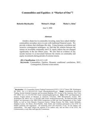
31. Figure1: Major Commodity and Equity Indices, 1991-2008
Note: Figure 1 plots the levels of four indices from January 2, 1991 to May 26, 2008: the Dow Jones
Industrial Average (DJIA) and the S&P 500 equity indices, and the Dow Jones DJ-AIG and S&P GSCI
commodity indices. The base level is set for January 2, 1991. The two equity indices (top two trends) tend
to move closely together. So do the two commodity indices – most of the time. Two exceptions are 1994-
1995 and 2006-2007, when the DJ-AIG index rose while the GSCI either stagnated or outright dropped in
value.
31

32. Figure 2A: Equity and Commodity Weekly Return Correlations: S&P 500 vs. GSCI, 1991-2008
Note: Figure 2A depicts estimates of the time-varying correlation between the weekly unlevered rates of
return (precisely, changes in log prices) on the S&P 500 (SP) and GSCI total return (GSTR) indices from
January 2, 1991 to May 26, 2008. The Figure provides plots for the following three estimation methods:
exponential smoother with 0.94 smoothing parameter (top left panel), rolling historical correlation (top
right) and dynamic conditional correlation by log-likehood for mean reverting model estimation (bottom
panel). The straight line running through each graph is the unconditional correlation from Table 2A.
32

33. Figure 2B:
Equity and Commodity Daily Return Correlations: S&P 500 vs. GSCI, 1991-2008
Note: Figure 2B depicts estimates of the time-varying correlation between the daily unlevered rates of
return (precisely, changes in log prices) on the S&P 500 (SP) and GSCI total return (GSTR) indices from
January 2, 1991 to May 26, 2007. The method used to compute estimates is dynamic conditional
correlation by log-likehood for mean reverting model estimation. The straight line running through each
graph is the unconditional correlation.
33

34. Figure 2C:
Equity and Commodity Monthly Return Correlations: S&P 500 vs. GSCI, 1991-2008
Note: Figure 2C depicts estimates of the time-varying correlation between the monthly unlevered rates of
return (precisely, changes in log prices) on the S&P 500 (SP) and GSCI total return (GSTR) indices from
January 2, 1991 to May 26, 2008. The method used to ompute estimates is dynamic conditional correlation
by log-likehood for mean reverting model estimation. The straight line running through each graph is the
unconditional correlation.
34

35. Figure 3A:
Equity and Commodity Weekly Return Correlations: S&P 500 vs. DJ-AIG, 1991-2008
Note: Figure 3A depicts estimates of the time-varying correlation between the weekly unlevered rates of
return (precisely, changes in log prices) on the S&P 500 (SP) and DJ-AIGCI total return (DJTR) indices
from January 2, 1991 to May 26, 2008. The Figure provides plots for the following three estimation
methods: exponential smoother with 0.94 smoothing parameter (top left panel), rolling historical
correlation (top right), and dynamic conditional correlation by log-likehood for mean reverting model
estimation (bottom panel). The straight line running through each graph is the unconditional correlation.
35

36. Figure 3B:
Equity and Commodity Daily Return Correlations: S&P 500 vs. DJ-AIG, 1991-2008
Note: Figure 3B depicts estimates of the time-varying correlation between the daily unlevered rates of
return (precisely, changes in log prices) on the S&P 500 (SP) and DJ-AIGCI total return (DJTR) indices
from January 2, 1991 to May 26, 2008. The method used to compute estimates is dynamic conditional
correlation by log-likehood for mean reverting model estimation. The straight line running through each
graph is the unconditional correlation.
36

37. Figure 3C:
Equity and Commodity Monthly Return Correlations: S&P 500 vs. DJ-AIG, 1991-2008
Note: Figure 3C depicts estimates of the time-varying correlation between the monthly unlevered rates of
return on the S&P 500 (SP) and DJ-AIGCI total return (DJTR) indices from January 2, 1991 to May 26,
2008. The method used to compute estimates is dynamic conditional correlation by log-likehood for mean
reverting model estimation. The straight line running through each graph is the unconditional correlation.
37

38. Figure 4:
Equity and Commodity Weekly Return Correlations: DJIA vs. GSCI, 1991-2008
Note: Figure 4 depicts estimates of the time-varying correlation between the weekly unlevered rates of
return (precisely, changes in log prices) on the Dow Jones Industrial Average (DJ) and GSCI total return
(GSTR) indices from January 2, 1991 to May 26, 2008. The Figure provides plots for the following three
estimation methods: exponential smoother with 0.94 smoothing parameter (top left panel), rolling historical
correlation (top right) and dynamic conditional correlation by log-likehood for mean reverting model
estimation (bottom panel). The straight line running through each graph is the unconditional correlation
from Table 2A.
38

39. Figure 5:
Equity and Commodity Weekly Return Correlations: DJIA vs. DJ-AIG, 1991-2008
Note: Figure 5 depicts estimates of the time-varying correlation between the weekly unlevered rates of
return (precisely, changes in log prices) on the Dow Jones Industrial Average (DJ) and DJ-AIGCI total
return (DJTR) indices from January 2, 1991 to May 26, 2008. The Figure provides plots for the following
three estimation methods: exponential smoother with 0.94 smoothing parameter (top left panel), rolling
historical correlation (top right) and dynamic conditional correlation by log-likehood for mean reverting
model estimation (bottom panel). The straight line running through each graph is the unconditional
correlation from Table 2A.
39