Predictive Statistics (Trending) a Tutorial por Ray Wicks
•
3 j'aime•658 vues

This document discusses predictive statistics and trend analysis techniques. It begins with an introduction to basic statistical concepts like linear regression analysis and examines how to calculate accuracy and the confidence interval of trend predictions. The document cautions that trend predictions assume the future will resemble the past and questions the assumptions behind trend analysis. It provides examples of how to perform linear regression calculations in Excel and SAS and discusses the impact of outliers on the regression fit.

Recommandé
Recommandé
Contenu connexe
Plus de Joao Galdino Mello de Souza
Plus de Joao Galdino Mello de Souza (20)
Dernier
Dernier (20)
Predictive Statistics (Trending) a Tutorial por Ray Wicks
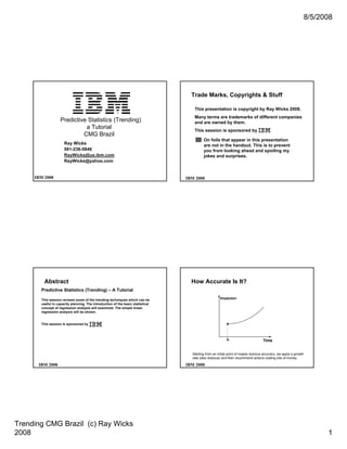
- 1. 8/5/2008 Trade Marks, Copyrights & Stuff This presentation is copyright by Ray Wicks 2008. Many terms are trademarks of different companies Predictive Statistics (Trending) and are owned by them. a Tutorial This session is sponsored by CMG Brazil On foils that appear in this presentation Ray Wicks are not in the handout. This is to prevent 561-236-5846 you from looking ahead and spoiling my RayWicks@us.ibm.com jokes and surprises. RayWicks@yahoo.com IBM 2008 IBM 2008 Abstract How Accurate Is It? Predictive Statistics (Trending) – A Tutorial This session reviews some of the trending techniques which can be Prediction useful in capacity planning. The introduction of the basic statistical concept of regression analysis will examined. The simple linear regression analysis will be shown. This session is sponsored by t0 Time Starting from an initial point of maybe dubious accuracy, we apply a growth rate (also dubious) and then recommend actions costing lots of money. IBM 2008 IBM 2008 Trending CMG Brazil (c) Ray Wicks 2008 1
- 2. 8/5/2008 Accuracy How Accurate Is It? Prediction Prediction Prediction p p t0 Time t0 Time t0 t Time t0 t Time At time t, is the prediction a precise point p or a fuzzy patch? Accuracy is found in values that are close to the expected curve. This closeness implies an expected bound or variation in reality. So a thicker line makes sense. IBM 2008 IBM 2008 Statistical Discourse Perceptual Structure A Conversation 0.45 You: The answer is 42.67. 0.4 0.35 =Normdist(x,0,1,0) 0.3 0.25 0.2 Them: I measured it and the answer is 42.663! 0.15 0.1 0.05 0 -4 -3 -2 -1 0 1 2 3 4 X You: Give me a break. Conceptual Structure Them: I just want to be exact. You: OK the answer is around 42.67. Them: How far around. You: ???? Blah, blah, blah IBM 2008 IBM 2008 Trending CMG Brazil (c) Ray Wicks 2008 2
- 3. 8/5/2008 Confidence Interval or How Thick is the Line? Confidence Interval Prediction 0.45 0.4 0.35 =Normdist(x,0,1,0) 0.3 0.25 0.2 Zα/2 [ μ – 1.96 σ/n , μ + 1.96 σ/n ] 0.15 t0 Time 0.1 [ μ – zα/2 σ/n , μ + zα/2 σ/n ] 0.05 0 -4 -3 -2 -1 0 1 2 3 4 X Using a Standard Normal Probability table, 95% confidence (2 tail) is found by looking P[m-2s < X < m+2s] = 0.954 for a z score of 0.025. P[m-1.96s < X < m+1.96s] = 0.95 or 95% In Excel: =Confidence(μ, σ, n) [L,U] is called the 100(1-α)% confidence interval. =Confidence(0.5,1,100) = 1.96 1-α is called the level of confidence associated with [L,U] IBM 2008 IBM 2008 Linear Regression (for Trending) Summary 1000 Given a list of numbers X={Xi} i=1 to n y = 3.0504x + 385.42 Statistics 900 Term Formula Excel PS View R2 = 0.7881 800 Count (number of items) n Number of points =Count(X) plotted 700 MIPS Used Average X=Sum(X)/n =Average(X) Center of gravity 600 Median§ X[ROUND DOWN 1+N*0.5] =MEDIAN(X) Middle number Variance 2 Spread of data 500 V=(Xi-X) )/n =Var(X) Standard Deviation s=SQRT(V) =Stnd(X) Spread of data 400 Coeficient of Variation Spread of data around 300 (Std/Avg) CV=s/X average Minimum First in Sorted list =MIN(X) Bottom of plot 200 Maximum Last in Sorted list =Max(X) Top of plot 100 Range Distance between top [Minimum,Maximum] and bottom 0 90th percentile§ X[ROUND DOWN 1+n*0.9] =Percentile(X,0.9) 10% from the top 0 50 100 150 200 Confidence interval Expected Variability of Look in book =Confidence(0.05,s,n) average (a thick line) Week §= Percentile formulae Obtain a useful fit of the data (y= mx+b) and then extend the values assume a sorted list; Low to high. of X to obtain predicted values of Y. But remember as Niels Bohr said: “Prediction is very hard to do. Especially about the future.” IBM 2008 IBM 2008 Trending CMG Brazil (c) Ray Wicks 2008 3
- 4. 8/5/2008 Trending Assumptions & Questions Reality 80 70 60 The future will be like the past. 1800 How much history is too much? 50 CPU% 40 30 1600 You should look at Era segments. 20 10 0 1400 0 10 20 30 40 50 60 70 80 90 100 110 120 130 140 150 Shape and scale of graph can be 1200 Week MIPS Used y = 3.0504x + 385.42 1000 interesting. 800 R2 = 0.7881 You may need more than 600 numbers.... The business and 400 technical environment? 200 0 Be smart and lazy…. What 0 50 100 150 200 questions are you answering? Week Linear regression’s predictions assume that the future looks like the past. IBM 2008 IBM 2008 Coding Implementation The Butterfly Effect Linear Fit for {Xi,Yi} Y Algorithm 1: Yi=B0 + B1Xi Xn+1 = s*Xn if Xn < 0.5 Yi Xn+1 = s*(1- Xn) otherwise e In Excel: cell Xn+1 is =IF(Xn<0.5, S*Xn, S*(1-Xn)) Y Algorithm 2: Yi Xn+1 = s *(0.5 - |Xn – 0.5|) B0 In Excel: cell Xn+1 is =S*(0.5-ABS(Xn-0.5)) X Xi Mathematically Equal. On the line would be perfect. (Yi - Y)2 (Ref. Chaos Under Control, section on Butterfly Effect.) Goodness of Fit R2 = Next to that would be a line (Yi - Y)2 with minimum error (e). Actually minimum e2 is better. IBM 2008 IBM 2008 Trending CMG Brazil (c) Ray Wicks 2008 4
- 5. 8/5/2008 Excel Help Correlation 7000 DASD I/O Rate 6000 5000 4000 Search Excel Help for R Squared return: 3000 2000 1000 RSQ: Returns the square of the Pearson product 0 moment correlation coefficient through data points 0 20 40 60 80 100 CPU% in known_y's and known_x's. For more information, see PEARSON. The r-squared value Correlation = COV(X,Y) / σx σy can be interpreted as the proportion of the variance in y attributable to the variance in x. = σxy2 / σx σy = E[(x-μx)(y-μy)] / σx σy Correlation [-1,1] =CORREL(CPU%,DASDIO) = 0.86 IBM 2008 IBM 2008 Briefly: Correlation is not Causality Causality & Correlation Claim: Eating Cheerios will lower your cholesterol Cause → Effect (sufficient cause) Cause → Effect ~Effect → ~Cause (necessary cause) Cause: Eating Cheerios Effect: Lower Cholesterol R2 or CORR(C,E) may indicate a linear Test: Real cause relationship without there being a causal Intervening Variable connection. Cheerios Lower Cholesterol In cities of various sizes: Bacon & Eggs Cholesterol C = number of TVs is highly correlated with E = number of murders. C = religious events is highly correlated with E = X Bacon & Eggs Lower Cholesterol number of suicides. There is a correlation between Eating Cheerios and lower Cholesterol but is there a causal relationship? IBM 2008 IBM 2008 Trending CMG Brazil (c) Ray Wicks 2008 5
- 6. 8/5/2008 Matrix Solution for Linear Fit B = (Mt * M)-1 * Mt * Y Excel Solution Solve for Y = B0 + B1*X X Y YH Sq (YH-YA) Sq (Y-YA) R2 80 M is 5x2 1 1.3 62.3 61.765 50.339025 43.0336 0.9262 =(SUM(F3:F7)/SUM(G3:G7)) y = 47.3x + 0.275 1 1.4 64.3 66.495 5.593225 20.7936 R2 = 0.9262 1 1.45 70.8 68.86 5.7678E-24 3.7636 75 1 1.5 71.1 71.225 5.593225 5.0176 1 1.6 75.8 75.955 50.339025 48.1636 Avg 68.86 70 CPU% MT is 2x5 1 1 1 1 1 ctl-shift-enter 1.3 1.4 1.45 1.5 1.6 65 MT*M is 2x2 5 7.25 7.25 10.563 60 INV(MTM) is 2x2 42.25 -29 -29 20 55 IMTM*MT is 2x5 4.55 1.65 0.2 -1.25 -4.15 -3 -1 0 1 3 50 IMTMMT*Y is 2x1 0.275 B0 1.2 1.3 1.4 1.5 1.6 1.7 47.3 B1 Units of Work IBM 2008 IBM 2008 Impact of Outlier A perfect fit is always possible 100 80 95 4 3 2 y = 58111x - 338194x + 736689x - 711801x + 257442 75 2 90 R =1 85 70 80 CPU% CPU% 75 65 y = -50.8x + 149.06 70 R2 = 0.2358 60 65 60 55 55 50 50 1.2 1.25 1.3 1.35 1.4 1.45 1.5 1.55 1.6 1.65 1.2 1.3 1.4 1.5 1.6 1.7 Units of Work Units of Work Albeit meaningless in this case. IBM 2008 IBM 2008 Trending CMG Brazil (c) Ray Wicks 2008 6
- 7. 8/5/2008 SAS Confidence of Fit. 85 y = 47.3x + 0.275 80 2 R = 0.9262 75 CPU% CPU% 70 LB UB 65 Linear (CPU%) 60 55 50 1.2 1.3 1.4 1.5 1.6 1.7 Units of Work IBM 2008 IBM 2008 Analyze -> Linear Regression Run Root MSE 1.72313 R-Square 0.9262 Dependent Mean 68.86000 Adj R-Sq 0.9017 Coeff Var 2.50236 Parameter Estimates Variable Label DF Parameter Standard t Value Pr > |t| Estimate Error Intercept Intercept 1 0.27500 11.20033 0.02 0.9820 X X 1 47.30000 7.70606 6.14 0.0087 IBM 2008 IBM 2008 Trending CMG Brazil (c) Ray Wicks 2008 7
- 8. 8/5/2008 Results Residuals For each Xi, plot e = Y- Yi Residual 10 5 Look for 0 random Residual 0 100 200 300 400 500 600 700 800 900 -5 distribution -10 around 0 -15 -20 Units of Work IBM 2008 IBM 2008 Regression other than Linear Interesting Case 40 0.0043x 40 y = 1.234e 35 35 2 y = 0.0335x R = 0.9457 30 30 2 R = 0.8569 CPU% CPU% 25 25 20 20 15 15 10 10 5 5 0 0 0 100 200 300 400 500 600 700 800 0 100 200 300 400 500 600 700 800 Blocks Blocks Notice the points are below the line until >600. Typical of DB/DC. Means less efficient as the load increases? The residuals have a pattern. That usually means a second level effect. Exponential fit is useful when computing compound growth IBM 2008 IBM 2008 Trending CMG Brazil (c) Ray Wicks 2008 8
- 9. 2008 05 /2 0.72 0.74 0.76 0.78 0.8 0.82 0.84 1/ 05 0 4 /2 0 0.1 0.2 0.3 0.4 0.5 0.6 0.7 0.8 0.9 8 /0 06 4 /0 4 /0 06 4 05/21/04 /1 IBM 2008 IBM 2008 1 /0 06 4 05/28/04 /1 8 /0 06 4 06/04/04 /2 5/ 06/11/04 07 0 4 /0 2/ 06/18/04 07 04 /0 9 /0 06/25/04 07 4 /1 6 /0 07/02/04 07 4 /2 (PS: It’s a line) 3 /0 07/09/04 07 4 /3 0 /0 07/16/04 08 4 /0 6/ 07/23/04 08 0 4 /1 3/ 04 07/30/04 08 /2 0 /0 08/06/04 08 4 /2 7 /0 08/13/04 09 4 PS to CS Dissonance /0 3 /0 08/20/04 09 4 /1 0 /0 08/27/04 09 4 /1 7/ 04 09/03/04 y = -0.0002x + 8.2996 09 /2 4/ 09/10/04 10 0 4 (PS: Polynomial fit looks good) /0 1 /0 09/17/04 4 R2 = 0.7817 (CS: fit looks good) 10 /0 8 /0 09/24/04 10 4 /1 5 /0 10/01/04 10 4 Trending CMG Brazil (c) Ray Wicks /2 2 /0 10/08/04 10 4 /2 10/15/04 9/ 11 0 4 /0 10/22/04 5 /0 4 y = -6E-08x3 + 0.0063x2 - 241.55x + 3E+06 10/29/04 R2 = 0.4388 (CS: Not a good line) 11/05/04 Perceptual to Conceptual Dissonance? 0 0.1 0.2 0.3 0.4 0.5 0.6 0.7 0.8 0.9 05/21/04 0.74 0.76 0.78 0.8 0.82 0.84 ??? 06/04/04 IBM 2008 IBM 2008 05/21/04 06/18/04 05/28/04 07/02/04 06/04/04 07/16/04 06/11/04 07/30/04 06/18/04 06/25/04 08/13/04 07/02/04 08/27/04 07/09/04 09/10/04 07/16/04 09/24/04 07/23/04 y = -0.0002x + 8.2996 10/08/04 07/30/04 08/06/04 10/22/04 08/13/04 11/05/04 08/20/04 11/19/04 08/27/04 12/03/04 09/03/04 12/17/04 09/10/04 09/17/04 12/31/04 09/24/04 01/14/05 10/01/04 01/28/05 10/08/04 02/11/05 10/15/04 In 144 Days, the $ will be worthless. 02/25/05 10/22/04 (PS: Visual Variability is scale dependent) 10/29/04 03/11/05 11/05/04 03/25/05 Perceptual to Conceptual Dissonance R2 = 0.4388 (CS: Variability is scale independent) 9 8/5/2008
- 10. 8/5/2008 Regression Analysis is not a Crystal Ball Philosophical Remark 1.37 Sensation 1.36 Negotiation 0.84 y= -0.0002x + 8.2996 2 R = 0.4388 0.83 1.35 0.82 0.81 0.8 0.79 0.78 1.34 0.77 0.76 0.75 0.74 1.33 (Lights Up) 1.32 1.31 Context 1.3 1.29 In reaching a conclusion, we negotiate between the 1.28 potential perceptual structures and the potential 1/18/07 2/7/07 2/27/07 3/19/07 4/8/07 4/28/07 5/18/07 6/7/07 6/27/07 7/17/07 conceptual structures and memory events. IBM 2008 IBM 2008 Model Building: Which is Best? Stepwise Results X1 X2 X3 X4 Y Stepwise Analysis 7 26 6 60 78.5 Table of Results for General Stepwise 1 29 15 52 74.3 X4 entered. 11 56 8 20 104.3 df SS MS F Significance F 11 31 8 47 87.6 Regression 1 1831.89616 1831.89616 22.7985202 0.000576232 7 52 6 33 95.9 Residual 11 883.8669169 80.3515379 Total 12 2715.763077 11 55 9 22 109.2 3 71 17 6 102.7 Coefficients Standard Error t Stat P-value Lower 95% Upper 95% 1 31 22 44 72.5 Intercept 117.5679312 5.262206511 22.34194552 1.62424E-10 105.9858927 129.1499696 X4 -0.738161808 0.154595996 -4.774779597 0.000576232 -1.078425302 -0.397898315 2 54 18 22 93.1 21 47 4 26 115.9 X1 entered. 1 40 23 34 83.8 11 66 9 12 113.3 df SS MS F Significance F Regression 2 2641.000965 1320.500482 176.6269631 1.58106E-08 10 68 8 12 109.4 Residual 10 74.76211216 7.476211216 Stepwise procedure to find the best combination of variables. Total 12 2715.763077 Y = b + a1X1 Intercept Coefficients Standard Error 103.0973816 t Stat 2.123983606 48.53963154 P-value 3.32434E-13 Lower 95% 98.36485126 Upper 95% 107.829912 Y = b + a1X1 + a2X2 X4 X1 -0.613953628 1.439958285 0.048644552 -12.62122063 0.13841664 10.40307211 1.81489E-07 1.10528E-06 -0.722340445 -0.505566811 1.131546793 1.748369777 Y = b + a2X2 + a3X3 …… No other variables could be entered into the model. Stepwise ends. Y = b + a1X1 + a2X2 + a3X3 + a4X4 Using Hald Data from Draper Using Add-In from Levine IBM 2008 IBM 2008 Trending CMG Brazil (c) Ray Wicks 2008 10