1. For a sample of 41 New England cities, a sociologist studies the crime rate in each city (crimes per 100,000 residents) as a function of its poverty rate (in %) and its median income (in $1,000s). The regression results are shown. ANOVA df SS MS F Significance F Regression 2 3,594,749 1,797,374.5 12.23270 1.5E-04 Residual 28 4,114,095 146,932.0 Total 30 7,708,844 a. Calculate the standard error of the estimate. (Round your answer to 2 decimal places.) formula877.mml b-1. What proportion of the variability in crime rate is explained by the variability in the explanatory variables? (Round your answer to 4 decimal places.) Explained proportion b-2. What proportion is unexplained? (Round your answer to 4 decimal places.) Unexplained proportion rev: 11_22_2013_QC_41534, 11_29_2013_QC_41646 2. In a multiple regression with two explanatory variables and 117 observations, it is found that SSR = 4.51 and SST = 8.86. a. Calculate the standard error of the estimate. (Round your answer to 2 decimal places.) se b. Calculate the coefficient of determination R2. (Round your answer to 4 decimal places.) R2 c. Calculate adjusted R2. (Round your answer to 4 decimal places.) Adjusted R2 rev: 09_16_2013_QC_34398 3. The following ANOVA table was obtained when estimating a multiple regression. ANOVA df SS MS F Significance F Regression 2 188,875.00 94,437.50 53.98 5.55E-10 Residual 26 45,484.65 1,749.41 Total 28 234,359.65 a. Calculate the standard error of the estimate. (Round your answer to 2 decimal places.) se b-1. Calculate the coefficient of determination. (Round your answer to 4 decimal places.) Coefficient of determination b-2. Interpret the coefficient of determination. The proportion of the variation in x that is explained by the regression model. The proportion of the variation in y that is explained by the regression model. c. Calculate adjusted R2. (Round your answer to 4 decimal places.) Adjusted R2 rev: 09_16_2013_QC_34398, 12_06_2013_QC_42096, 12_18_2014_QC_CS-890 4. The homeownership rate in the United States was 67.4% in 2009. In order to determine if homeownership is linked with income, 2009 state level data on the homeownership rate (Ownership) and median household income (Income) were collected. The data can be found on the text website, labeled Home Ownership. State Income Ownership Alabama $38,990 72.3% Alaska $60,614 65.7% Arizona $44,749 67.4% Arkansas $35,548 66.6% California $55,144 56.0% Colorado $54,940 67.2% Connecticut $63,861 69.4% Delaware $51,124 75.0% District of Columbia $52,151 44.1% Florida $44,641 69.4% Georgia $42,350 65.9% Hawaii $54,659 58.4% Idaho $45,788 73.9% Illinois $51,880 67.8% Indiana $43,315 70.4% ...

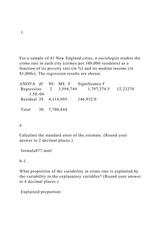
1. 1.
For a sample of 41 New England cities, a sociologist studies the
crime rate in each city (crimes per 100,000 residents) as a
function of its poverty rate (in %) and its median income (in
$1,000s). The regression results are shown.
ANOVA df SS MS F Significance F
Regression 2 3,594,749 1,797,374.5 12.23270
1.5E-04
Residual 28 4,114,095 146,932.0
Total 30 7,708,844
a.
Calculate the standard error of the estimate. (Round your
answer to 2 decimal places.)
formula877.mml
b-1.
What proportion of the variability in crime rate is explained by
the variability in the explanatory variables? (Round your answer
to 4 decimal places.)
Explained proportion

2. b-2.
What proportion is unexplained? (Round your answer to 4
decimal places.)
Unexplained proportion
rev: 11_22_2013_QC_41534, 11_29_2013_QC_41646
2.
In a multiple regression with two explanatory variables and 117
observations, it is found that SSR = 4.51 and SST = 8.86.
a. Calculate the standard error of the estimate. (Round your
answer to 2 decimal places.)
se
b. Calculate the coefficient of determination R2. (Round your
answer to 4 decimal places.)
R2

3. c. Calculate adjusted R2. (Round your answer to 4 decimal
places.)
Adjusted R2
rev: 09_16_2013_QC_34398
3.
The following ANOVA table was obtained when estimating a
multiple regression.
ANOVA df SS MS F Significance F
Regression 2 188,875.00 94,437.50 53.98
5.55E-10
Residual 26 45,484.65 1,749.41
Total 28 234,359.65
a. Calculate the standard error of the estimate. (Round your
answer to 2 decimal places.)
se

4. b-1. Calculate the coefficient of determination. (Round your
answer to 4 decimal places.)
Coefficient of determination
b-2. Interpret the coefficient of determination.
The proportion of the variation in x that is explained by
the regression model.
The proportion of the variation in y that is explained by
the regression model.
c. Calculate adjusted R2. (Round your answer to 4 decimal
places.)
Adjusted R2
rev: 09_16_2013_QC_34398, 12_06_2013_QC_42096,
12_18_2014_QC_CS-890
4.
The homeownership rate in the United States was 67.4% in
2009. In order to determine if homeownership is linked with
income, 2009 state level data on the homeownership rate
(Ownership) and median household income (Income) were

5. collected. The data can be found on the text website, labeled
Home Ownership.
State
Income
Ownership
Alabama
$38,990
72.3%
Alaska
$60,614
65.7%
Arizona
$44,749
67.4%

6. Arkansas
$35,548
66.6%
California
$55,144
56.0%
Colorado
$54,940
67.2%
Connecticut
$63,861
69.4%
Delaware
$51,124

7. 75.0%
District of Columbia
$52,151
44.1%
Florida
$44,641
69.4%
Georgia
$42,350
65.9%
Hawaii
$54,659
58.4%

8. Idaho
$45,788
73.9%
Illinois
$51,880
67.8%
Indiana
$43,315
70.4%
Iowa
$49,731
71.0%
Kansas
$43,727

9. 65.9%
Kentucky
$41,674
69.5%
Louisiana
$44,443
70.3%
Maine
$46,512
72.5%
Maryland
$63,196
68.5%

10. Massachusetts
$58,383
64.0%
Michigan
$45,004
72.9%
Minnesota
$55,100
71.6%
Mississippi
$34,088
73.4%
Missouri
$47,779

11. 70.5%
Montana
$39,447
69.0%
Nebraska
$48,605
68.8%
Nevada
$50,444
61.2%
New Hampshire
$63,141
74.8%

12. New Jersey
$63,787
64.9%
New Mexico
$42,552
67.5%
New York
$49,226
53.3%
North Carolina
$40,916
68.4%
North Dakota
$49,085

13. 64.4%
Ohio
$44,889
68.2%
Oklahoma
$44,888
68.1%
Oregon
$48,108
66.8%
Pennsylvania
$47,182
70.7%

14. Rhode Island
$50,644
61.7%
South Carolina
$40,111
72.6%
South Dakota
$44,836
68.1%
Tennessee
$39,527
69.4%
Texas
$46,485

15. 64.0%
Utah
$57,501
72.8%
Vermont
$51,328
72.9%
Virginia
$59,511
68.6%
Washington
$59,402
64.4%

16. West Virginia
$39,500
76.8%
Wisconsin
$50,247
69.0%
Wyoming
$51,480
72.4%
SOURCE: www.census.gov
PictureClick here for the Excel Data File
State
Income ($)
Ownership (%)
Alabama
38,990
72.3
Alaska
60,614

17. 65.7
Arizona
44,749
67.4
Arkansas
35,548
66.6
California
55,144
56.0
Colorado
54,940
67.2
Connecticut
63,861
69.4
Delaware
51,124
75.0
District of Columbia
52,151
44.1
Florida
44,641
69.4
Georgia
42,350
65.9
Hawaii
54,659
58.4
Idaho
45,788
73.9
Illinois
51,880

18. 67.8
Indiana
43,315
70.4
Iowa
49,731
71.0
Kansas
43,727
65.9
Kentucky
41,674
69.5
Louisiana
44,443
70.3
Maine
46,512
72.5
Maryland
63,196
68.5
Massachusetts
58,383
64.0
Michigan
45,004
72.9
Minnesota
55,100
71.6
Mississippi
34,088
73.4
Missouri
47,779

19. 70.5
Montana
39,447
69.0
Nebraska
48,605
68.8
Nevada
50,444
61.2
New Hampshire
63,141
74.8
New Jersey
63,787
64.9
New Mexico
42,552
67.5
New York
49,226
53.3
North Carolina
40,916
68.4
North Dakota
49,085
64.4
Ohio
44,889
68.2
Oklahoma
44,888
68.1
Oregon
48,108

20. 66.8
Pennsylvania
47,182
70.7
Rhode Island
50,644
61.7
South Carolina
40,111
72.6
South Dakota
44,836
68.1
Tennessee
39,527
69.4
Texas
46,485
64.0
Utah
57,501
72.8
Vermont
51,328
72.9
Virginia
59,511
68.6
Washington
59,402
64.4
West Virginia
39,500
76.8
Wisconsin
50,247

21. 69.0
Wyoming
51,480
72.4
a-1.
Estimate the model Ownership = β0 + β1Income + ε. (Negative
values should be indicated by a minus sign. Round your answers
to 4 decimal places.)
y-hat = + Income

22. a-2. Interpret the model.
For a $1,000 increase in income, homeownership rate is
predicted to decrease by 0.02%.
For a $1,000 increase in income, homeownership rate is
predicted to increase by 0.02%.
For a $1,000 decrease in income, homeownership rate is
predicted to increase by 0.01%.
For a $1,000 decrease in income, homeownership rate is
predicted to decrease by 0.01%.
b. What is the standard error of the estimate? (Round your
answer to 2 decimal places.)
se
c. Interpret the coefficient of determination.
4.63% of the sample variation in y is explained by the
estimated regression equation.
4.63% of the sample variation in x is explained by the
estimated regression equation.
3.63% of the sample variation in x is explained by the
estimated regression equation.
5.63% of the sample variation in y is explained by the
estimated regression equation.
rev: 09_16_2013_QC_34398, 11_01_2013_QC_34398
5.
Consider the following sample data:

23. x 26 32 16 31 10 30 34 32
y 35 53 40 38 28 47 29 35
PictureClick here for the Excel Data File
x
26
32
16
31
10
30
34
32
y
35
53
40
38
28
47
29
35
b.
Calculate b1 and b0. What is the sample regression equation?
(Round intermediate calculations to 4 decimal places and final
answers to 2 decimal places.)
y-hat = + x

24. c.
Find the predicted value for y if x equals 18, 23, and 28. (Round
intermediate coefficient values and final answers to 2 decimal
places.)
y-hat
If x = 18
If x = 23
If x = 28
rev: 09_16_2013_QC_34398, 10_31_2013_QC_34398,
11_21_2013_QC_34398, 12_17_2013_QC_34398
6.
In a simple linear regression based on 28 observations, it is
found that b1 = 7.1 and se(bj) = 1.9. Consider the hypotheses
(Use Table 2):
H0: β1 ≥ 10 and HA: β1 < 10
a.
At the 5% significance level, find the critical value(s).
(Negative value should be indicated by a minus sign. Round
your answer to 3 decimal places.)

25. Critical value
b.
Calculate the value of the appropriate test statistic. (Negative
value should be indicated by a minus sign. Round your answer
to 2 decimal places.)
Test statistic
c. At the 5% significance level, what is the conclusion to the
hypothesis test? Is the slope coefficient less than 10?
Do not reject H0Picture the slope coefficient is not less
than 10.
Reject H0Picture the slope coefficient is less than 10.
Do not reject H0Picture the slope coefficient is less than
10.
Reject H0Picture the slope coefficient is not less than 10.
rev: 11_01_2013_QC_34398
7.
Using data from 50 workers, a researcher estimates Wage = β0
+ β1 Education + β2 Experience +β3 Age + ε, where Wage is
the hourly wage rate and Education, Experience, and Age are
the years of higher education, the years of experience, and the
age of the worker, respectively. A portion of the regression
results is shown in the following table.
Coefficients Standard Error t Stat p-value

26. Intercept 7.95 4.29 1.19 0.0641
Education 1.87 0.40 3.51 0.0002
Experience 0.48 0.19 3.34 0.0027
Age −0.01 0.06 −0.19 0.7170
a-1. What is the point estimate for β1?
1.87
0.48
a-2. Interpret this value.
As Education increases by 1 unit, Wage is predicted to
increase by 1.87 units.
As Education increases by 1 unit, Wage is predicted to
increase by 0.48 units, holding Age and Experience constant.
As Education increases by 1 unit, Wage is predicted to
increase by 0.48 units.
As Education increases by 1 unit, Wage is predicted to
increase by 1.87 units, holding Age and Experience constant.
a-3. What is the point estimate for β2?
0.48
1.87
a-4. Interpret this value.

27. Same interpretation by using 1.87 or -0.01
As Experience increases by 1 unit, Wage is predicted to
increase by 0.48 units, holding Age and Education constant.
b.
What is the sample regression equation? (Negative value should
be indicated by a minus sign. Round your answers to 2 decimal
places.)
y-hat = + Education + Experience + Age
c.
What is the predicted value for Age = 23, Education = 4 and
Experience = 2. (Do not round intermediate calculations. Round
your answer to 2 decimal places.)
y-hat
rev: 09_16_2013_QC_34398
8.
A social scientist would like to analyze the relationship between

28. educational attainment and salary. He collects the following
sample data, where Education refers to years of higher
education and Salary is the individual’s annual salary in
thousands of dollars:
Education 3 4 6 2 5 4 8 0
Salary $40 36 56 35 72 47 107 52
PictureClick here for the Excel Data File
Education
3
4
6
2
5
4
8
0
Salary
40
36
56
35
72
47
107
52
a.
Find the sample regression equation for the model: Salary = β0
+ β1Education + ε. (Round intermediate calculations to 4
decimal places. Enter your answers in thousands rounded to 2

29. decimal places.)
formula537.mml + Education
b. Interpret the coefficient for education.
As Education increases by 1 unit, an individual’s annual
salary is predicted to decrease by $7,000.
As Education increases by 1 unit, an individual’s annual
salary is predicted to increase by $8,000.
As Education increases by 1 unit, an individual’s annual
salary is predicted to increase by $7,000.
As Education inceases by 1 unit, an individual’s annual
salary is predicted to decrease by $8,000.
c.
What is the predicted salary for an individual who completed 7
years of higher education? (Round intermediate coefficient
values to 2 decimal places and final answer, in dollars, to the
nearest whole number.)
formula723.mml $
rev: 09_16_2013_QC_34398, 10_31_2013_QC_34398
9.
Consider the following simple linear regression results based on
20 observations. Use Table 2.

30. Coefficients Standard Error t Stat p-value Lower
95% Upper 95%
Intercept 30.7705 4.6589 6.6047 0.0000 20.98
40.56
x1 0.1071 0.1879 0.5700 0.5757 −0.29 0.50
a-1. Choose the hypotheses to determine if the intercept differs
from zero.
H0: β0 ≥ 0; HA: β0 < 0
H0: β0 ≤ 0; HA: β0 > 0
H0: β0 = 0; HA: β0 ≠ 0
a-2. At the 5% significance level, what is the conclusion to the
hypothesis test? Does the intercept differ from zero?
Do not reject H0Picture the intercept differs from zero.
Do not reject H0Picture the intercept is greater than zero.
Reject H0Picture the intercept differs from zero.
Reject H0Picture the intercept is greater than zero.
b-1.
Construct the 95% confidence interval for the slope coefficient.
(Negative values should be indicated by a minus sign. Round
your intermediate calculations to 4 decimal places,"tα/2,df"

31. value to 3 decimal places and final answers to 2 decimal
places.)
Confidence interval to
b-2.
At the 5% significance level, does the slope differ from zero?
No, since the interval contains zero.
Yes, since the interval does not contain zero.
Yes, since the interval contains zero.
No, since the interval does not contain zero.
rev: 11_01_2013_QC_34398, 11_30_2013_QC_41780
10.
In a simple linear regression, the following information is
given:
formula321.mml = − 29; formula726.mml= 48;
formula323.mml
formula324.mml

32. a.
Calculate b1. (Negative value should be indicated by a minus
sign. Round your answer to 2 decimal places.)
b1
b.
Calculate b0. (Round intermediate calculations to 4 decimal
places and final answer to 2 decimal places.)
b0
c-1.
What is the sample regression equation? (Negative value should
be indicated by a minus sign. Round your answers to 2 decimal
places.)
y-hat = + x
c-2.
Predict y if x equals −21.(Round intermediate coefficient values
and final answer to 2 decimal places.)
y-hat
rev: 09_17_2013_QC_34398, 10_31_2013_QC_34398