Test

4

Classification:
Basic Concepts,
Decision Trees, and
Model Evaluation
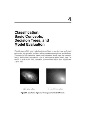
Classification, which is the task of assigning objects to one of several predefined
categories, is a pervasive problem that encompasses many diverse applications.
Examples include detecting spam email messages based upon the message
header and content, categorizing cells as malignant or benign based upon the
results of MRI scans, and classifying galaxies based upon their shapes (see
Figure 4.1).

(a) A spiral galaxy. (b) An elliptical galaxy.

Figure 4.1. Classification of galaxies. The images are from the NASA website.

146 Chapter 4 Classification

Input Output

Classification
Attribute set Class label
model
(x) (y)

Figure 4.2. Classification as the task of mapping an input attribute set x into its class label y.

This chapter introduces the basic concepts of classification, describes some
of the key issues such as model overfitting, and presents methods for evaluating
and comparing the performance of a classification technique. While it focuses
mainly on a technique known as decision tree induction, most of the discussion
in this chapter is also applicable to other classification techniques, many of
which are covered in Chapter 5.

4.1 Preliminaries
The input data for a classification task is a collection of records. Each record,
also known as an instance or example, is characterized by a tuple (x, y), where
x is the attribute set and y is a special attribute, designated as the class label
(also known as category or target attribute). Table 4.1 shows a sample data set
used for classifying vertebrates into one of the following categories: mammal,
bird, fish, reptile, or amphibian. The attribute set includes properties of a
vertebrate such as its body temperature, skin cover, method of reproduction,
ability to fly, and ability to live in water. Although the attributes presented
in Table 4.1 are mostly discrete, the attribute set can also contain continuous
features. The class label, on the other hand, must be a discrete attribute.
This is a key characteristic that distinguishes classification from regression,
a predictive modeling task in which y is a continuous attribute. Regression
techniques are covered in Appendix D.
Definition 4.1 (Classification). Classification is the task of learning a tar-
get function f that maps each attribute set x to one of the predefined class
labels y.
The target function is also known informally as a classification model.
A classification model is useful for the following purposes.

Descriptive Modeling A classification model can serve as an explanatory
tool to distinguish between objects of different classes. For example, it would
be useful—for both biologists and others—to have a descriptive model that

4.1 Preliminaries 147

Table 4.1. The vertebrate data set.

Name Body Skin Gives Aquatic Aerial Has Hiber- Class
Temperature Cover Birth Creature Creature Legs nates Label
human warm-blooded hair yes no no yes no mammal
python cold-blooded scales no no no no yes reptile
salmon cold-blooded scales no yes no no no fish
whale warm-blooded hair yes yes no no no mammal
frog cold-blooded none no semi no yes yes amphibian
komodo cold-blooded scales no no no yes no reptile
dragon
bat warm-blooded hair yes no yes yes yes mammal
pigeon warm-blooded feathers no no yes yes no bird
cat warm-blooded fur yes no no yes no mammal
leopard cold-blooded scales yes yes no no no fish
shark
turtle cold-blooded scales no semi no yes no reptile
penguin warm-blooded feathers no semi no yes no bird
porcupine warm-blooded quills yes no no yes yes mammal
eel cold-blooded scales no yes no no no fish
salamander cold-blooded none no semi no yes yes amphibian

summarizes the data shown in Table 4.1 and explains what features define a
vertebrate as a mammal, reptile, bird, fish, or amphibian.

Predictive Modeling A classification model can also be used to predict
the class label of unknown records. As shown in Figure 4.2, a classification
model can be treated as a black box that automatically assigns a class label
when presented with the attribute set of an unknown record. Suppose we are
given the following characteristics of a creature known as a gila monster:

Name Body Skin Gives Aquatic Aerial Has Hiber- Class
Temperature Cover Birth Creature Creature Legs nates Label
gila monster cold-blooded scales no no no yes yes ?

We can use a classification model built from the data set shown in Table 4.1
to determine the class to which the creature belongs.

Classification techniques are most suited for predicting or describing data
sets with binary or nominal categories. They are less effective for ordinal
categories (e.g., to classify a person as a member of high-, medium-, or low-
income group) because they do not consider the implicit order among the
categories. Other forms of relationships, such as the subclass–superclass re-
lationships among categories (e.g., humans and apes are primates, which in


turn, is a subclass of mammals) are also ignored. The remainder of this chapter
focuses only on binary or nominal class labels.

4.2 General Approach to Solving a Classification
Problem
A classification technique (or classifier) is a systematic approach to building
classification models from an input data set. Examples include decision tree
classifiers, rule-based classifiers, neural networks, support vector machines,
and na¨ Bayes classifiers. Each technique employs a learning algorithm
ıve
to identify a model that best fits the relationship between the attribute set and
class label of the input data. The model generated by a learning algorithm
should both fit the input data well and correctly predict the class labels of
records it has never seen before. Therefore, a key objective of the learning
algorithm is to build models with good generalization capability; i.e., models
that accurately predict the class labels of previously unknown records.
Figure 4.3 shows a general approach for solving classification problems.
First, a training set consisting of records whose class labels are known must

Training Set
Tid Attrib1 Attrib2 Attrib3 Class Learning
1 Yes Large 125K No Algorithm
2 No Medium 100K No
3 No Small 70K No
4 Yes Medium 120K No
Induction
5 No Large 95K Yes
6 No Medium 60K No
7 Yes Large 220K No Learn
8 No Small 85K Yes Model
9 No Medium 75K No
10 No Small 90K Yes
Model

Test Set Apply
Tid Attrib1 Attrib2 Attrib3 Class
Model
11 No Small 55K ?
12 Yes Medium 80K ? Deduction
13 Yes Large 110K ?
14 No Small 95K ?
15 No Large 67K ?

Figure 4.3. General approach for building a classification model.

4.2 General Approach to Solving a Classification Problem 149

Table 4.2. Confusion matrix for a 2-class problem.
Predicted Class
Class = 1 Class = 0
Actual Class = 1 f11 f10
Class Class = 0 f01 f00

be provided. The training set is used to build a classification model, which is
subsequently applied to the test set, which consists of records with unknown
class labels.
Evaluation of the performance of a classification model is based on the
counts of test records correctly and incorrectly predicted by the model. These
counts are tabulated in a table known as a confusion matrix. Table 4.2
depicts the confusion matrix for a binary classification problem. Each entry
fij in this table denotes the number of records from class i predicted to be
of class j. For instance, f01 is the number of records from class 0 incorrectly
predicted as class 1. Based on the entries in the confusion matrix, the total
number of correct predictions made by the model is (f11 + f00 ) and the total
number of incorrect predictions is (f10 + f01 ).
Although a confusion matrix provides the information needed to determine
how well a classification model performs, summarizing this information with
a single number would make it more convenient to compare the performance
of different models. This can be done using a performance metric such as
accuracy, which is defined as follows:

Number of correct predictions f11 + f00
Accuracy = = . (4.1)
Total number of predictions f11 + f10 + f01 + f00

Equivalently, the performance of a model can be expressed in terms of its
error rate, which is given by the following equation:

Number of wrong predictions f10 + f01
Error rate = = . (4.2)
Total number of predictions f11 + f10 + f01 + f00

Most classification algorithms seek models that attain the highest accuracy, or
equivalently, the lowest error rate when applied to the test set. We will revisit
the topic of model evaluation in Section 4.5.


4.3 Decision Tree Induction
This section introduces a decision tree classifier, which is a simple yet widely
used classification technique.

4.3.1 How a Decision Tree Works
To illustrate how classification with a decision tree works, consider a simpler
version of the vertebrate classification problem described in the previous sec-
tion. Instead of classifying the vertebrates into five distinct groups of species,
we assign them to two categories: mammals and non-mammals.
Suppose a new species is discovered by scientists. How can we tell whether
it is a mammal or a non-mammal? One approach is to pose a series of questions
about the characteristics of the species. The first question we may ask is
whether the species is cold- or warm-blooded. If it is cold-blooded, then it is
definitely not a mammal. Otherwise, it is either a bird or a mammal. In the
latter case, we need to ask a follow-up question: Do the females of the species
give birth to their young? Those that do give birth are definitely mammals,
while those that do not are likely to be non-mammals (with the exception of
egg-laying mammals such as the platypus and spiny anteater).
The previous example illustrates how we can solve a classification problem
by asking a series of carefully crafted questions about the attributes of the
test record. Each time we receive an answer, a follow-up question is asked
until we reach a conclusion about the class label of the record. The series of
questions and their possible answers can be organized in the form of a decision
tree, which is a hierarchical structure consisting of nodes and directed edges.
Figure 4.4 shows the decision tree for the mammal classification problem. The
tree has three types of nodes:
• A root node that has no incoming edges and zero or more outgoing
edges.

• Internal nodes, each of which has exactly one incoming edge and two
or more outgoing edges.

• Leaf or terminal nodes, each of which has exactly one incoming edge
and no outgoing edges.
In a decision tree, each leaf node is assigned a class label. The non-
terminal nodes, which include the root and other internal nodes, contain
attribute test conditions to separate records that have different characteris-
tics. For example, the root node shown in Figure 4.4 uses the attribute Body

4.3 Decision Tree Induction 151

Body
Temperature Root
node

Internal Warm Cold
node

Non-
Gives Birth mammals

Yes No

Leaf
Non- nodes
Mammals
mammals

Figure 4.4. A decision tree for the mammal classification problem.

Temperature to separate warm-blooded from cold-blooded vertebrates. Since
all cold-blooded vertebrates are non-mammals, a leaf node labeled Non-mammals
is created as the right child of the root node. If the vertebrate is warm-blooded,
a subsequent attribute, Gives Birth, is used to distinguish mammals from
other warm-blooded creatures, which are mostly birds.
Classifying a test record is straightforward once a decision tree has been
constructed. Starting from the root node, we apply the test condition to the
record and follow the appropriate branch based on the outcome of the test.
This will lead us either to another internal node, for which a new test condition
is applied, or to a leaf node. The class label associated with the leaf node is
then assigned to the record. As an illustration, Figure 4.5 traces the path in
the decision tree that is used to predict the class label of a flamingo. The path
terminates at a leaf node labeled Non-mammals.

4.3.2 How to Build a Decision Tree
In principle, there are exponentially many decision trees that can be con-
structed from a given set of attributes. While some of the trees are more accu-
rate than others, finding the optimal tree is computationally infeasible because
of the exponential size of the search space. Nevertheless, efficient algorithms
have been developed to induce a reasonably accurate, albeit suboptimal, de-
cision tree in a reasonable amount of time. These algorithms usually employ
a greedy strategy that grows a decision tree by making a series of locally op-


Unlabeled Name Body temperature Gives Birth ... Class
data Flamingo Warm No ... ?

Body Non-
Temperature mammals

Warm Cold

Non-
Gives Birth mammals

Yes No

Non-
Mammals
mammals

Figure 4.5. Classifying an unlabeled vertebrate. The dashed lines represent the outcomes of applying
various attribute test conditions on the unlabeled vertebrate. The vertebrate is eventually assigned to
the Non-mammal class.

timum decisions about which attribute to use for partitioning the data. One
such algorithm is Hunt’s algorithm, which is the basis of many existing de-
cision tree induction algorithms, including ID3, C4.5, and CART. This section
presents a high-level discussion of Hunt’s algorithm and illustrates some of its
design issues.

Hunt’s Algorithm
In Hunt’s algorithm, a decision tree is grown in a recursive fashion by parti-
tioning the training records into successively purer subsets. Let Dt be the set
of training records that are associated with node t and y = {y1 , y2 , . . . , yc } be
the class labels. The following is a recursive deﬁnition of Hunt’s algorithm.

Step 1: If all the records in Dt belong to the same class yt , then t is a leaf
node labeled as yt .

Step 2: If Dt contains records that belong to more than one class, an at-
tribute test condition is selected to partition the records into smaller
subsets. A child node is created for each outcome of the test condi-
tion and the records in Dt are distributed to the children based on the
outcomes. The algorithm is then recursively applied to each child node.


al us
ic uo
ry or
g tin ss
na te n a
bi ca co cl
Home Marital Annual Defaulted
Tid
Owner Status Income Borrower
1 Yes Single 125K No
2 No Married 100K No
3 No Single 70K No
4 Yes Married 120K No
5 No Divorced 95K Yes
6 No Married 60K No
7 Yes Divorced 220K No
8 No Single 85K Yes
9 No Married 75K No
10 No Single 90K Yes

Figure 4.6. Training set for predicting borrowers who will default on loan payments.

To illustrate how the algorithm works, consider the problem of predicting
whether a loan applicant will repay her loan obligations or become delinquent,
subsequently defaulting on her loan. A training set for this problem can be
constructed by examining the records of previous borrowers. In the example
shown in Figure 4.6, each record contains the personal information of a bor-
rower along with a class label indicating whether the borrower has defaulted
on loan payments.
The initial tree for the classification problem contains a single node with
class label Defaulted = No (see Figure 4.7(a)), which means that most of
the borrowers successfully repaid their loans. The tree, however, needs to be
refined since the root node contains records from both classes. The records are
subsequently divided into smaller subsets based on the outcomes of the Home
Owner test condition, as shown in Figure 4.7(b). The justification for choosing
this attribute test condition will be discussed later. For now, we will assume
that this is the best criterion for splitting the data at this point. Hunt’s
algorithm is then applied recursively to each child of the root node. From
the training set given in Figure 4.6, notice that all borrowers who are home
owners successfully repaid their loans. The left child of the root is therefore a
leaf node labeled Defaulted = No (see Figure 4.7(b)). For the right child, we
need to continue applying the recursive step of Hunt’s algorithm until all the
records belong to the same class. The trees resulting from each recursive step
are shown in Figures 4.7(c) and (d).


Home
Owner
Yes No
Defaulted = No
Defaulted = No Defaulted = No

(a) (b)

Home
Owner
Yes No

Home Defaulted = No Marital
Owner Status
Yes No Single, Married
Divorced
Defaulted = No Marital Annual Defaulted = No
Status Income
Single, Married < 80K >= 80K
Divorced
Defaulted = Yes Defaulted = No Defaulted = No Defaulted = Yes

(c) (d)

Figure 4.7. Hunt’s algorithm for inducing decision trees.

Hunt’s algorithm will work if every combination of attribute values is
present in the training data and each combination has a unique class label.
These assumptions are too stringent for use in most practical situations. Ad-
ditional conditions are needed to handle the following cases:

1. It is possible for some of the child nodes created in Step 2 to be empty;
i.e., there are no records associated with these nodes. This can happen
if none of the training records have the combination of attribute values
associated with such nodes. In this case the node is declared a leaf
node with the same class label as the majority class of training records
associated with its parent node.

2. In Step 2, if all the records associated with Dt have identical attribute
values (except for the class label), then it is not possible to split these
records any further. In this case, the node is declared a leaf node with
the same class label as the majority class of training records associated
with this node.


Design Issues of Decision Tree Induction
A learning algorithm for inducing decision trees must address the following
two issues.

1. How should the training records be split? Each recursive step
of the tree-growing process must select an attribute test condition to
divide the records into smaller subsets. To implement this step, the
algorithm must provide a method for specifying the test condition for
different attribute types as well as an objective measure for evaluating
the goodness of each test condition.

2. How should the splitting procedure stop? A stopping condition is
needed to terminate the tree-growing process. A possible strategy is to
continue expanding a node until either all the records belong to the same
class or all the records have identical attribute values. Although both
conditions are sufficient to stop any decision tree induction algorithm,
other criteria can be imposed to allow the tree-growing procedure to
terminate earlier. The advantages of early termination will be discussed
later in Section 4.4.5.

4.3.3 Methods for Expressing Attribute Test Conditions
Decision tree induction algorithms must provide a method for expressing an
attribute test condition and its corresponding outcomes for different attribute
types.

Binary Attributes The test condition for a binary attribute generates two
potential outcomes, as shown in Figure 4.8.

Body
Temperature

Warm- Cold-
blooded blooded

Figure 4.8. Test condition for binary attributes.


Marital
Status

Single Divorced Married
(a) Multiway split

Marital Marital Marital
Status Status Status

OR OR

{Married} {Single, {Single} {Married, {Single, {Divorced}
Divorced} Divorced} Married}

(b) Binary split {by grouping attribute values}

Figure 4.9. Test conditions for nominal attributes.

Nominal Attributes Since a nominal attribute can have many values, its
test condition can be expressed in two ways, as shown in Figure 4.9. For
a multiway split (Figure 4.9(a)), the number of outcomes depends on the
number of distinct values for the corresponding attribute. For example, if
an attribute such as marital status has three distinct values—single, married,
or divorced—its test condition will produce a three-way split. On the other
hand, some decision tree algorithms, such as CART, produce only binary splits
by considering all 2k−1 − 1 ways of creating a binary partition of k attribute
values. Figure 4.9(b) illustrates three diﬀerent ways of grouping the attribute
values for marital status into two subsets.

Ordinal Attributes Ordinal attributes can also produce binary or multiway
splits. Ordinal attribute values can be grouped as long as the grouping does
not violate the order property of the attribute values. Figure 4.10 illustrates
various ways of splitting training records based on the Shirt Size attribute.
The groupings shown in Figures 4.10(a) and (b) preserve the order among
the attribute values, whereas the grouping shown in Figure 4.10(c) violates
this property because it combines the attribute values Small and Large into


Shirt Shirt Shirt
Size Size Size

{Small, {Large, {Small} {Medium, Large, {Small, {Medium,
Medium} Extra Large} Extra Large} Large} Extra Large}

(a) (b) (c)

Figure 4.10. Different ways of grouping ordinal attribute values.

the same partition while Medium and Extra Large are combined into another
partition.

Continuous Attributes For continuous attributes, the test condition can
be expressed as a comparison test (A < v) or (A ≥ v) with binary outcomes, or
a range query with outcomes of the form vi ≤ A < vi+1 , for i = 1, . . . , k. The
diﬀerence between these approaches is shown in Figure 4.11. For the binary
case, the decision tree algorithm must consider all possible split positions v,
and it selects the one that produces the best partition. For the multiway
split, the algorithm must consider all possible ranges of continuous values.
One approach is to apply the discretization strategies described in Section
2.3.6 on page 57. After discretization, a new ordinal value will be assigned to
each discretized interval. Adjacent intervals can also be aggregated into wider
ranges as long as the order property is preserved.

Annual
Income Annual
> 80K Income

< 10K > 80K
Yes No

{10K, 25K} {25K, 50K} {50K, 80K}
(a) (b)

Figure 4.11. Test condition for continuous attributes.


Car Customer
Gender
Type ID

Male Female Family Luxury v1 v20
v10 v11
Sports

C0: 6 C0: 4 C0:1 C0: 8 C0: 1 C0: 1 . . . C0: 1 C0: 0 . . . C0: 0
C1: 4 C1: 6 C1: 3 C1: 0 C1: 7 C1: 0 C1: 0 C1: 1 C1: 1
(a) (b) (c)

Figure 4.12. Multiway versus binary splits.

4.3.4 Measures for Selecting the Best Split
There are many measures that can be used to determine the best way to split
the records. These measures are deﬁned in terms of the class distribution of
the records before and after splitting.
Let p(i|t) denote the fraction of records belonging to class i at a given node
t. We sometimes omit the reference to node t and express the fraction as pi .
In a two-class problem, the class distribution at any node can be written as
(p0 , p1 ), where p1 = 1 − p0 . To illustrate, consider the test conditions shown
in Figure 4.12. The class distribution before splitting is (0.5, 0.5) because
there are an equal number of records from each class. If we split the data
using the Gender attribute, then the class distributions of the child nodes are
(0.6, 0.4) and (0.4, 0.6), respectively. Although the classes are no longer evenly
distributed, the child nodes still contain records from both classes. Splitting
on the second attribute, Car Type, will result in purer partitions.
The measures developed for selecting the best split are often based on the
degree of impurity of the child nodes. The smaller the degree of impurity, the
more skewed the class distribution. For example, a node with class distribu-
tion (0, 1) has zero impurity, whereas a node with uniform class distribution
(0.5, 0.5) has the highest impurity. Examples of impurity measures include

c−1
Entropy(t) = − p(i|t) log2 p(i|t), (4.3)
i=0
c−1
Gini(t) = 1 − [p(i|t)]2 , (4.4)
i=0
Classiﬁcation error(t) = 1 − max[p(i|t)], (4.5)
i

where c is the number of classes and 0 log2 0 = 0 in entropy calculations.


1

0.9
Entropy
0.8

0.7

0.6

0.5
Gini
0.4

0.3

0.2 Misclassification error

0.1

0
0 0.1 0.2 0.3 0.4 0.5 0.6 0.7 0.8 0.9 1
p

Figure 4.13. Comparison among the impurity measures for binary classification problems.

Figure 4.13 compares the values of the impurity measures for binary classi-
fication problems. p refers to the fraction of records that belong to one of the
two classes. Observe that all three measures attain their maximum value when
the class distribution is uniform (i.e., when p = 0.5). The minimum values for
the measures are attained when all the records belong to the same class (i.e.,
when p equals 0 or 1). We next provide several examples of computing the
different impurity measures.

Node N1 Count Gini = 1 − (0/6)2 − (6/6)2 = 0
Class=0 0 Entropy = −(0/6) log2 (0/6) − (6/6) log2 (6/6) = 0
Class=1 6 Error = 1 − max[0/6, 6/6] = 0

Node N2 Count Gini = 1 − (1/6)2 − (5/6)2 = 0.278
Class=0 1 Entropy = −(1/6) log2 (1/6) − (5/6) log2 (5/6) = 0.650
Class=1 5 Error = 1 − max[1/6, 5/6] = 0.167

Node N3 Count Gini = 1 − (3/6)2 − (3/6)2 = 0.5
Class=0 3 Entropy = −(3/6) log2 (3/6) − (3/6) log2 (3/6) = 1
Class=1 3 Error = 1 − max[3/6, 3/6] = 0.5


The preceding examples, along with Figure 4.13, illustrate the consistency
among different impurity measures. Based on these calculations, node N1 has
the lowest impurity value, followed by N2 and N3 . Despite their consistency,
the attribute chosen as the test condition may vary depending on the choice
of impurity measure, as will be shown in Exercise 3 on page 198.
To determine how well a test condition performs, we need to compare the
degree of impurity of the parent node (before splitting) with the degree of
impurity of the child nodes (after splitting). The larger their difference, the
better the test condition. The gain, ∆, is a criterion that can be used to
determine the goodness of a split:

k
N (vj )
∆ = I(parent) − I(vj ), (4.6)
N
j=1

where I(·) is the impurity measure of a given node, N is the total number of
records at the parent node, k is the number of attribute values, and N (vj )
is the number of records associated with the child node, vj . Decision tree
induction algorithms often choose a test condition that maximizes the gain
∆. Since I(parent) is the same for all test conditions, maximizing the gain is
equivalent to minimizing the weighted average impurity measures of the child
nodes. Finally, when entropy is used as the impurity measure in Equation 4.6,
the difference in entropy is known as the information gain, ∆info .

Splitting of Binary Attributes
Consider the diagram shown in Figure 4.14. Suppose there are two ways to
split the data into smaller subsets. Before splitting, the Gini index is 0.5 since
there are an equal number of records from both classes. If attribute A is chosen
to split the data, the Gini index for node N1 is 0.4898, and for node N2, it
is 0.480. The weighted average of the Gini index for the descendent nodes is
(7/12) × 0.4898 + (5/12) × 0.480 = 0.486. Similarly, we can show that the
weighted average of the Gini index for attribute B is 0.375. Since the subsets
for attribute B have a smaller Gini index, it is preferred over attribute A.

Splitting of Nominal Attributes
As previously noted, a nominal attribute can produce either binary or multi-
way splits, as shown in Figure 4.15. The computation of the Gini index for a
binary split is similar to that shown for determining binary attributes. For the
first binary grouping of the Car Type attribute, the Gini index of {Sports,


Parent
C0 6
C1 6
Gini = 0.500
A B

Yes No Yes No

Node N1 Node N2 Node N1 Node N2

N1 N2 N1 N2
C0 4 2 C0 1 5
C1 3 3 C1 4 2
Gini = 0.486 Gini = 0.375

Figure 4.14. Splitting binary attributes.

Car Type Car Type Car Type
{Sports, {Family, Family Luxury
Luxury} {Family} Luxury} {Sports}
Sports

Car Type Car Type Car Type
{Sports, {Family,
{Family} {Sports} Family Sports Luxury
Luxury} Luxury}
C0 9 1 C0 8 2 C0 1 8 1
C1 7 3 C1 0 10 C1 3 0 7
Gini 0.468 Gini 0.167 Gini 0.163

(a) Binary split (b) Multiway split

Figure 4.15. Splitting nominal attributes.

Luxury} is 0.4922 and the Gini index of {Family} is 0.3750. The weighted
average Gini index for the grouping is equal to

16/20 × 0.4922 + 4/20 × 0.3750 = 0.468.

Similarly, for the second binary grouping of {Sports} and {Family, Luxury},
the weighted average Gini index is 0.167. The second grouping has a lower
Gini index because its corresponding subsets are much purer.


Class No No No Yes Yes Yes No No No No
Annual Income
Sorted Values 60 70 75 85 90 95 100 120 125 220

Split Positions 55 65 72 80 87 92 97 110 122 172 230
<= > <= > <= > <= > <= > <= > <= > <= > <= > <= > <= >
Yes 0 3 0 3 0 3 0 3 1 2 2 1 3 0 3 0 3 0 3 0 3 0
No 0 7 1 6 2 5 3 4 3 4 3 4 3 4 4 3 5 2 6 1 7 0
Gini 0.420 0.400 0.375 0.343 0.417 0.400 0.300 0.343 0.375 0.400 0.420

Figure 4.16. Splitting continuous attributes.

For the multiway split, the Gini index is computed for every attribute value.
Since Gini({Family}) = 0.375, Gini({Sports}) = 0, and Gini({Luxury}) =
0.219, the overall Gini index for the multiway split is equal to

4/20 × 0.375 + 8/20 × 0 + 8/20 × 0.219 = 0.163.

The multiway split has a smaller Gini index compared to both two-way splits.
This result is not surprising because the two-way split actually merges some
of the outcomes of a multiway split, and thus, results in less pure subsets.

Splitting of Continuous Attributes
Consider the example shown in Figure 4.16, in which the test condition Annual
Income ≤ v is used to split the training records for the loan default classifica-
tion problem. A brute-force method for finding v is to consider every value of
the attribute in the N records as a candidate split position. For each candidate
v, the data set is scanned once to count the number of records with annual
income less than or greater than v. We then compute the Gini index for each
candidate and choose the one that gives the lowest value. This approach is
computationally expensive because it requires O(N ) operations to compute
the Gini index at each candidate split position. Since there are N candidates,
the overall complexity of this task is O(N 2 ). To reduce the complexity, the
training records are sorted based on their annual income, a computation that
requires O(N log N ) time. Candidate split positions are identified by taking
the midpoints between two adjacent sorted values: 55, 65, 72, and so on. How-
ever, unlike the brute-force approach, we do not have to examine all N records
when evaluating the Gini index of a candidate split position.
For the first candidate, v = 55, none of the records has annual income less
than $55K. As a result, the Gini index for the descendent node with Annual


Income < $55K is zero. On the other hand, the number of records with annual
income greater than or equal to $55K is 3 (for class Yes) and 7 (for class No),
respectively. Thus, the Gini index for this node is 0.420. The overall Gini
index for this candidate split position is equal to 0 × 0 + 1 × 0.420 = 0.420.
For the second candidate, v = 65, we can determine its class distribution
by updating the distribution of the previous candidate. More specifically, the
new distribution is obtained by examining the class label of the record with
the lowest annual income (i.e., $60K). Since the class label for this record is
No, the count for class No is increased from 0 to 1 (for Annual Income ≤ $65K)
and is decreased from 7 to 6 (for Annual Income > $65K). The distribution
for class Yes remains unchanged. The new weighted-average Gini index for
this candidate split position is 0.400.
This procedure is repeated until the Gini index values for all candidates are
computed, as shown in Figure 4.16. The best split position corresponds to the
one that produces the smallest Gini index, i.e., v = 97. This procedure is less
expensive because it requires a constant amount of time to update the class
distribution at each candidate split position. It can be further optimized by
considering only candidate split positions located between two adjacent records
with different class labels. For example, because the first three sorted records
(with annual incomes $60K, $70K, and $75K) have identical class labels, the
best split position should not reside between $60K and $75K. Therefore, the
candidate split positions at v = $55K, $65K, $72K, $87K, $92K, $110K, $122K,
$172K, and $230K are ignored because they are located between two adjacent
records with the same class labels. This approach allows us to reduce the
number of candidate split positions from 11 to 2.

Gain Ratio
Impurity measures such as entropy and Gini index tend to favor attributes that
have a large number of distinct values. Figure 4.12 shows three alternative
test conditions for partitioning the data set given in Exercise 2 on page 198.
Comparing the first test condition, Gender, with the second, Car Type, it
is easy to see that Car Type seems to provide a better way of splitting the
data since it produces purer descendent nodes. However, if we compare both
conditions with Customer ID, the latter appears to produce purer partitions.
Yet Customer ID is not a predictive attribute because its value is unique for
each record. Even in a less extreme situation, a test condition that results in a
large number of outcomes may not be desirable because the number of records
associated with each partition is too small to enable us to make any reliable
predictions.


There are two strategies for overcoming this problem. The ﬁrst strategy is
to restrict the test conditions to binary splits only. This strategy is employed
by decision tree algorithms such as CART. Another strategy is to modify the
splitting criterion to take into account the number of outcomes produced by
the attribute test condition. For example, in the C4.5 decision tree algorithm,
a splitting criterion known as gain ratio is used to determine the goodness
of a split. This criterion is deﬁned as follows:

∆info
Gain ratio = . (4.7)
Split Info

Here, Split Info = − k P (vi ) log2 P (vi ) and k is the total number of splits.
i=1
For example, if each attribute value has the same number of records, then
∀i : P (vi ) = 1/k and the split information would be equal to log2 k. This
example suggests that if an attribute produces a large number of splits, its
split information will also be large, which in turn reduces its gain ratio.

4.3.5 Algorithm for Decision Tree Induction
A skeleton decision tree induction algorithm called TreeGrowth is shown
in Algorithm 4.1. The input to this algorithm consists of the training records
E and the attribute set F . The algorithm works by recursively selecting the
best attribute to split the data (Step 7) and expanding the leaf nodes of the

Algorithm 4.1 A skeleton decision tree induction algorithm.
TreeGrowth (E, F )
1: if stopping cond(E,F ) = true then
2: leaf = createNode().
3: leaf.label = Classify(E).
4: return leaf .
5: else
6: root = createNode().
7: root.test cond = find best split(E, F ).
8: let V = {v|v is a possible outcome of root.test cond }.
9: for each v ∈ V do
10: Ev = {e | root.test cond(e) = v and e ∈ E}.
11: child = TreeGrowth(Ev , F ).
12: add child as descendent of root and label the edge (root → child) as v.
13: end for
14: end if
15: return root.


tree (Steps 11 and 12) until the stopping criterion is met (Step 1). The details
of this algorithm are explained below:

1. The createNode() function extends the decision tree by creating a new
node. A node in the decision tree has either a test condition, denoted as
node.test cond, or a class label, denoted as node.label.

2. The find best split() function determines which attribute should be
selected as the test condition for splitting the training records. As pre-
viously noted, the choice of test condition depends on which impurity
measure is used to determine the goodness of a split. Some widely used
measures include entropy, the Gini index, and the χ2 statistic.

3. The Classify() function determines the class label to be assigned to a
leaf node. For each leaf node t, let p(i|t) denote the fraction of training
records from class i associated with the node t. In most cases, the leaf
node is assigned to the class that has the majority number of training
records:
leaf.label = argmax p(i|t), (4.8)
i

where the argmax operator returns the argument i that maximizes the
expression p(i|t). Besides providing the information needed to determine
the class label of a leaf node, the fraction p(i|t) can also be used to es-
timate the probability that a record assigned to the leaf node t belongs
to class i. Sections 5.7.2 and 5.7.3 describe how such probability esti-
mates can be used to determine the performance of a decision tree under
different cost functions.

4. The stopping cond() function is used to terminate the tree-growing pro-
cess by testing whether all the records have either the same class label
or the same attribute values. Another way to terminate the recursive
function is to test whether the number of records have fallen below some
minimum threshold.

After building the decision tree, a tree-pruning step can be performed
to reduce the size of the decision tree. Decision trees that are too large are
susceptible to a phenomenon known as overfitting. Pruning helps by trim-
ming the branches of the initial tree in a way that improves the generalization
capability of the decision tree. The issues of overfitting and tree pruning are
discussed in more detail in Section 4.4.


Session IP Address Timestamp Request Requested Web Page Protocol Status Number Referrer User Agent
Method of Bytes
1 160.11.11.11 08/Aug/2004 GET http://www.cs.umn.edu/ HTTP/1.1 200 6424 Mozilla/4.0
10:15:21 ~kumar (compatible; MSIE 6.0;
Windows NT 5.0)
1 160.11.11.11 08/Aug/2004 GET http://www.cs.umn.edu/ HTTP/1.1 200 41378 http://www.cs.umn.edu/ Mozilla/4.0
10:15:34 ~kumar/MINDS ~kumar (compatible; MSIE 6.0;
Windows NT 5.0)
10:15:41 ~kumar/MINDS/MINDS ~kumar/MINDS (compatible; MSIE 6.0;
_papers.htm Windows NT 5.0)
10:16:11 ~kumar/papers/papers. ~kumar (compatible; MSIE 6.0;
html Windows NT 5.0)
2 35.9.2.2 08/Aug/2004 GET http://www.cs.umn.edu/ HTTP/1.0 200 3149 Mozilla/5.0 (Windows; U;
10:16:15 ~steinbac Windows NT 5.1; en-US;
rv:1.7) Gecko/20040616

(a) Example of a Web server log.

Attribute Name Description
totalPages Total number of pages retrieved in a Web session
http://www.cs.umn.edu/~kumar ImagePages Total number of image pages retrieved in a Web session
TotalTime Total amount of time spent by Web site visitor
RepeatedAccess The same page requested more than once in a Web session
ErrorRequest Errors in requesting for Web pages
GET Percentage of requests made using GET method
MINDS
POST Percentage of requests made using POST method
papers/papers.html
HEAD Percentage of requests made using HEAD method
Breadth Breadth of Web traversal
Depth Depth of Web traversal
MultilP Session with multiple IP addresses
MINDS/MINDS_papers.htm
MultiAgent Session with multiple user agents

(b) Graph of a Web session. (c) Derived attributes for Web robot detection.

Figure 4.17. Input data for Web robot detection.

4.3.6 An Example: Web Robot Detection
Web usage mining is the task of applying data mining techniques to extract
useful patterns from Web access logs. These patterns can reveal interesting
characteristics of site visitors; e.g., people who repeatedly visit a Web site and
view the same product description page are more likely to buy the product if
certain incentives such as rebates or free shipping are oﬀered.
In Web usage mining, it is important to distinguish accesses made by hu-
man users from those due to Web robots. A Web robot (also known as a Web
crawler) is a software program that automatically locates and retrieves infor-
mation from the Internet by following the hyperlinks embedded in Web pages.
These programs are deployed by search engine portals to gather the documents
necessary for indexing the Web. Web robot accesses must be discarded before
applying Web mining techniques to analyze human browsing behavior.


This section describes how a decision tree classifier can be used to distin-
guish between accesses by human users and those by Web robots. The input
data was obtained from a Web server log, a sample of which is shown in Figure
4.17(a). Each line corresponds to a single page request made by a Web client
(a user or a Web robot). The fields recorded in the Web log include the IP
address of the client, timestamp of the request, Web address of the requested
document, size of the document, and the client’s identity (via the user agent
field). A Web session is a sequence of requests made by a client during a single
visit to a Web site. Each Web session can be modeled as a directed graph, in
which the nodes correspond to Web pages and the edges correspond to hyper-
links connecting one Web page to another. Figure 4.17(b) shows a graphical
representation of the first Web session given in the Web server log.
To classify the Web sessions, features are constructed to describe the char-
acteristics of each session. Figure 4.17(c) shows some of the features used
for the Web robot detection task. Among the notable features include the
depth and breadth of the traversal. Depth determines the maximum dis-
tance of a requested page, where distance is measured in terms of the num-
ber of hyperlinks away from the entry point of the Web site. For example,
the home page http://www.cs.umn.edu/∼kumar is assumed to be at depth
0, whereas http://www.cs.umn.edu/kumar/MINDS/MINDS papers.htm is lo-
cated at depth 2. Based on the Web graph shown in Figure 4.17(b), the depth
attribute for the first session is equal to two. The breadth attribute measures
the width of the corresponding Web graph. For example, the breadth of the
Web session shown in Figure 4.17(b) is equal to two.
The data set for classification contains 2916 records, with equal numbers
of sessions due to Web robots (class 1) and human users (class 0). 10% of the
data were reserved for training while the remaining 90% were used for testing.
The induced decision tree model is shown in Figure 4.18. The tree has an
error rate equal to 3.8% on the training set and 5.3% on the test set.
The model suggests that Web robots can be distinguished from human
users in the following way:

1. Accesses by Web robots tend to be broad but shallow, whereas accesses
by human users tend to be more focused (narrow but deep).

2. Unlike human users, Web robots seldom retrieve the image pages asso-
ciated with a Web document.

3. Sessions due to Web robots tend to be long and contain a large number
of requested pages.


Decision Tree:
depth = 1:
| breadth> 7 : class 1
| breadth<= 7:
| | breadth <= 3:
| | | ImagePages> 0.375: class 0
| | | ImagePages<= 0.375:
| | | | totalPages<= 6: class 1
| | | | totalPages> 6:
| | | | | breadth <= 1: class 1
| | | | | breadth > 1: class 0
| | width > 3:
| | | MultilP = 0:
| | | | ImagePages<= 0.1333: class 1
| | | | ImagePages> 0.1333:
| | | | breadth <= 6: class 0
| | | | breadth > 6: class 1
| | | MultilP = 1:
| | | | TotalTime <= 361: class 0
| | | | TotalTime > 361: class 1
depth> 1:
| MultiAgent = 0:
| | depth > 2: class 0
| | depth < 2:
| | | MultilP = 1: class 0
| | | MultilP = 0:
| | | | breadth <= 6: class 0
| | | | breadth > 6:
| | | | | RepeatedAccess <= 0.322: class 0
| | | | | RepeatedAccess > 0.322: class 1
| MultiAgent = 1:
| | totalPages <= 81: class 0
| | totalPages > 81: class 1

Figure 4.18. Decision tree model for Web robot detection.

4. Web robots are more likely to make repeated requests for the same doc-
ument since the Web pages retrieved by human users are often cached
by the browser.

4.3.7 Characteristics of Decision Tree Induction
The following is a summary of the important characteristics of decision tree
induction algorithms.

1. Decision tree induction is a nonparametric approach for building classiﬁ-
cation models. In other words, it does not require any prior assumptions
regarding the type of probability distributions satisﬁed by the class and
other attributes (unlike some of the techniques described in Chapter 5).


2. Finding an optimal decision tree is an NP-complete problem. Many de-
cision tree algorithms employ a heuristic-based approach to guide their
search in the vast hypothesis space. For example, the algorithm pre-
sented in Section 4.3.5 uses a greedy, top-down, recursive partitioning
strategy for growing a decision tree.

3. Techniques developed for constructing decision trees are computationally
inexpensive, making it possible to quickly construct models even when
the training set size is very large. Furthermore, once a decision tree has
been built, classifying a test record is extremely fast, with a worst-case
complexity of O(w), where w is the maximum depth of the tree.

4. Decision trees, especially smaller-sized trees, are relatively easy to inter-
pret. The accuracies of the trees are also comparable to other classifica-
tion techniques for many simple data sets.

5. Decision trees provide an expressive representation for learning discrete-
valued functions. However, they do not generalize well to certain types
of Boolean problems. One notable example is the parity function, whose
value is 0 (1) when there is an odd (even) number of Boolean attributes
with the value T rue. Accurate modeling of such a function requires a full
decision tree with 2d nodes, where d is the number of Boolean attributes
(see Exercise 1 on page 198).

6. Decision tree algorithms are quite robust to the presence of noise, espe-
cially when methods for avoiding overfitting, as described in Section 4.4,
are employed.

7. The presence of redundant attributes does not adversely affect the ac-
curacy of decision trees. An attribute is redundant if it is strongly cor-
related with another attribute in the data. One of the two redundant
attributes will not be used for splitting once the other attribute has been
chosen. However, if the data set contains many irrelevant attributes, i.e.,
attributes that are not useful for the classification task, then some of the
irrelevant attributes may be accidently chosen during the tree-growing
process, which results in a decision tree that is larger than necessary.
Feature selection techniques can help to improve the accuracy of deci-
sion trees by eliminating the irrelevant attributes during preprocessing.
We will investigate the issue of too many irrelevant attributes in Section
4.4.3.


8. Since most decision tree algorithms employ a top-down, recursive parti-
tioning approach, the number of records becomes smaller as we traverse
down the tree. At the leaf nodes, the number of records may be too
small to make a statistically significant decision about the class rep-
resentation of the nodes. This is known as the data fragmentation
problem. One possible solution is to disallow further splitting when the
number of records falls below a certain threshold.

9. A subtree can be replicated multiple times in a decision tree, as illus-
trated in Figure 4.19. This makes the decision tree more complex than
necessary and perhaps more difficult to interpret. Such a situation can
arise from decision tree implementations that rely on a single attribute
test condition at each internal node. Since most of the decision tree al-
gorithms use a divide-and-conquer partitioning strategy, the same test
condition can be applied to different parts of the attribute space, thus
leading to the subtree replication problem.

P

Q R

S 0 Q 1

0 1 S 0

0 1

Figure 4.19. Tree replication problem. The same subtree can appear at different branches.

10. The test conditions described so far in this chapter involve using only a
single attribute at a time. As a consequence, the tree-growing procedure
can be viewed as the process of partitioning the attribute space into
disjoint regions until each region contains records of the same class (see
Figure 4.20). The border between two neighboring regions of different
classes is known as a decision boundary. Since the test condition in-
volves only a single attribute, the decision boundaries are rectilinear; i.e.,
parallel to the “coordinate axes.” This limits the expressiveness of the


1
0.9
x < 0.43
0.8
0.7 Yes No
0.6
0.5
y

y < 0.47 y < 0.33
0.4
0.3 Yes No Yes No

0.2 :4 :0 :0 :4
0.1 :0 :4 :3 :0
0
0 0.1 0.2 0.3 0.4 0.5 0.6 0.7 0.8 0.9 1
x

Figure 4.20. Example of a decision tree and its decision boundaries for a two-dimensional data set.

1

0.9

0.8

0.7

0.6

0.5

0.4

0.3

0.2

0.1

0
0 0.1 0.2 0.3 0.4 0.5 0.6 0.7 0.8 0.9 1

Figure 4.21. Example of data set that cannot be partitioned optimally using test conditions involving
single attributes.

decision tree representation for modeling complex relationships among
continuous attributes. Figure 4.21 illustrates a data set that cannot be
classiﬁed eﬀectively by a decision tree algorithm that uses test conditions
involving only a single attribute at a time.


An oblique decision tree can be used to overcome this limitation
because it allows test conditions that involve more than one attribute.
The data set given in Figure 4.21 can be easily represented by an oblique
decision tree containing a single node with test condition

x + y < 1.

Although such techniques are more expressive and can produce more
compact trees, finding the optimal test condition for a given node can
be computationally expensive.
Constructive induction provides another way to partition the data
into homogeneous, nonrectangular regions (see Section 2.3.5 on page 57).
This approach creates composite attributes representing an arithmetic
or logical combination of the existing attributes. The new attributes
provide a better discrimination of the classes and are augmented to the
data set prior to decision tree induction. Unlike the oblique decision tree
approach, constructive induction is less expensive because it identifies all
the relevant combinations of attributes once, prior to constructing the
decision tree. In contrast, an oblique decision tree must determine the
right attribute combination dynamically, every time an internal node is
expanded. However, constructive induction can introduce attribute re-
dundancy in the data since the new attribute is a combination of several
existing attributes.
11. Studies have shown that the choice of impurity measure has little effect
on the performance of decision tree induction algorithms. This is because
many impurity measures are quite consistent with each other, as shown
in Figure 4.13 on page 159. Indeed, the strategy used to prune the
tree has a greater impact on the final tree than the choice of impurity
measure.

4.4 Model Overfitting
The errors committed by a classification model are generally divided into two
types: training errors and generalization errors. Training error, also
known as resubstitution error or apparent error, is the number of misclas-
sification errors committed on training records, whereas generalization error
is the expected error of the model on previously unseen records.
Recall from Section 4.2 that a good classification model must not only fit
the training data well, it must also accurately classify records it has never

4.4 Model Overfitting 173

Training set
20

18

16

14

12
x2

10

8

6

4

2

0
0 2 4 6 8 10 12 14 16 18 20
x1

Figure 4.22. Example of a data set with binary classes.

seen before. In other words, a good model must have low training error as
well as low generalization error. This is important because a model that fits
the training data too well can have a poorer generalization error than a model
with a higher training error. Such a situation is known as model overfitting.

Overfitting Example in Two-Dimensional Data For a more concrete
example of the overfitting problem, consider the two-dimensional data set
shown in Figure 4.22. The data set contains data points that belong to two
different classes, denoted as class o and class +, respectively. The data points
for the o class are generated from a mixture of three Gaussian distributions,
while a uniform distribution is used to generate the data points for the + class.
There are altogether 1200 points belonging to the o class and 1800 points be-
longing to the + class. 30% of the points are chosen for training, while the
remaining 70% are used for testing. A decision tree classifier that uses the
Gini index as its impurity measure is then applied to the training set. To
investigate the effect of overfitting, different levels of pruning are applied to
the initial, fully-grown tree. Figure 4.23(b) shows the training and test error
rates of the decision tree.


0.4

Training Error
0.35 Test Error

0.3

0.25
Error Rate
0.2

0.15

0.1

0.05

0
0 50 100 150 200 250 300
Number of Nodes

Figure 4.23. Training and test error rates.

Notice that the training and test error rates of the model are large when the
size of the tree is very small. This situation is known as model underfitting.
Underfitting occurs because the model has yet to learn the true structure of
the data. As a result, it performs poorly on both the training and the test
sets. As the number of nodes in the decision tree increases, the tree will have
fewer training and test errors. However, once the tree becomes too large, its
test error rate begins to increase even though its training error rate continues
to decrease. This phenomenon is known as model overfitting.
To understand the overfitting phenomenon, note that the training error of
a model can be reduced by increasing the model complexity. For example, the
leaf nodes of the tree can be expanded until it perfectly fits the training data.
Although the training error for such a complex tree is zero, the test error can
be large because the tree may contain nodes that accidently fit some of the
noise points in the training data. Such nodes can degrade the performance
of the tree because they do not generalize well to the test examples. Figure
4.24 shows the structure of two decision trees with different number of nodes.
The tree that contains the smaller number of nodes has a higher training error
rate, but a lower test error rate compared to the more complex tree.
Overfitting and underfitting are two pathologies that are related to the
model complexity. The remainder of this section examines some of the poten-
tial causes of model overfitting.


x2 < 12.63
x2 < 17.35
x1 < 13.29

x1 < 6.56 x1 < 2.15
x2 < 19.93

x1 < 7.24
x2 < 8.64

x1 < 3.03 x1 < 12.11
x2 < 12.63 x2 < 1.38
x1 < 6.78
x2 < 12.68
x1 < 13.29 x2 < 17.35 x1 < 2.72 x1 < 18.88
x2 < 4.06

x1 < 6.56 x1 < 2.15 x2 < 15.77 x2 < 17.14
x1 < 6.99

x2 < 12.89
x1 < 7.24
x2 < 8.64
x2 < 13.80

x1 < 12.11
x2 < 1.38 x2 < 16.75

x1 < 18.88
x2 < 16.33

(a) Decision tree with 11 leaf (b) Decision tree with 24 leaf nodes.
nodes.

Figure 4.24. Decision trees with different model complexities.

4.4.1 Overfitting Due to Presence of Noise
Consider the training and test sets shown in Tables 4.3 and 4.4 for the mammal
classification problem. Two of the ten training records are mislabeled: bats
and whales are classified as non-mammals instead of mammals.
A decision tree that perfectly fits the training data is shown in Figure
4.25(a). Although the training error for the tree is zero, its error rate on

Table 4.3. An example training set for classifying mammals. Class labels with asterisk symbols repre-
sent mislabeled records.

Name Body Gives Four- Hibernates Class
Temperature Birth legged Label
porcupine warm-blooded yes yes yes yes
cat warm-blooded yes yes no yes
bat warm-blooded yes no yes no∗
whale warm-blooded yes no no no∗
salamander cold-blooded no yes yes no
komodo dragon cold-blooded no yes no no
python cold-blooded no no yes no
salmon cold-blooded no no no no
eagle warm-blooded no no no no
guppy cold-blooded yes no no no


Table 4.4. An example test set for classifying mammals.
human warm-blooded yes no no yes
pigeon warm-blooded no no no no
elephant warm-blooded yes yes no yes
leopard shark cold-blooded yes no no no
turtle cold-blooded no yes no no
penguin cold-blooded no no no no
eel cold-blooded no no no no
dolphin warm-blooded yes no no yes
spiny anteater warm-blooded no yes yes yes
gila monster cold-blooded no yes yes no

Body Body
Temperature Temperature

Warm-blooded Cold-blooded Warm-blooded Cold-blooded

Non- Non-
Gives Birth mammals Gives Birth mammals

Yes No Yes No

Four- Non- Non-
Mammals
legged mammals mammals

Yes No

Non-
Mammals
mammals

(a) Model M1 (b) Model M2

Figure 4.25. Decision tree induced from the data set shown in Table 4.3.

the test set is 30%. Both humans and dolphins were misclassiﬁed as non-
mammals because their attribute values for Body Temperature, Gives Birth,
and Four-legged are identical to the mislabeled records in the training set.
Spiny anteaters, on the other hand, represent an exceptional case in which the
class label of a test record contradicts the class labels of other similar records
in the training set. Errors due to exceptional cases are often unavoidable and
establish the minimum error rate achievable by any classiﬁer.


In contrast, the decision tree M 2 shown in Figure 4.25(b) has a lower test
error rate (10%) even though its training error rate is somewhat higher (20%).
It is evident that the first decision tree, M 1, has overfitted the training data
because there is a simpler model with lower error rate on the test set. The
Four-legged attribute test condition in model M 1 is spurious because it fits
the mislabeled training records, which leads to the misclassification of records
in the test set.

4.4.2 Overfitting Due to Lack of Representative Samples
Models that make their classification decisions based on a small number of
training records are also susceptible to overfitting. Such models can be gener-
ated because of lack of representative samples in the training data and learning
algorithms that continue to refine their models even when few training records
are available. We illustrate these effects in the example below.
Consider the five training records shown in Table 4.5. All of these training
records are labeled correctly and the corresponding decision tree is depicted
in Figure 4.26. Although its training error is zero, its error rate on the test
set is 30%.

Table 4.5. An example training set for classifying mammals.
salamander cold-blooded no yes yes no
guppy cold-blooded yes no no no
eagle warm-blooded no no no no
poorwill warm-blooded no no yes no
platypus warm-blooded no yes yes yes

Humans, elephants, and dolphins are misclassified because the decision tree
classifies all warm-blooded vertebrates that do not hibernate as non-mammals.
The tree arrives at this classification decision because there is only one training
record, which is an eagle, with such characteristics. This example clearly
demonstrates the danger of making wrong predictions when there are not
enough representative examples at the leaf nodes of a decision tree.


Body
Temperature

Warm-blooded Cold-blooded

Non-
Hibernates mammals

Yes No

Four- Non-
legged mammals

Yes No

Non-
Mammals
mammals

Figure 4.26. Decision tree induced from the data set shown in Table 4.5.

4.4.3 Overfitting and the Multiple Comparison Procedure
Model overfitting may arise in learning algorithms that employ a methodology
known as multiple comparison procedure. To understand multiple comparison
procedure, consider the task of predicting whether the stock market will rise
or fall in the next ten trading days. If a stock analyst simply makes random
guesses, the probability that her prediction is correct on any trading day is
0.5. However, the probability that she will predict correctly at least eight out
of the ten times is
10 10 10
8 + 9 + 10
= 0.0547,
210
which seems quite unlikely.
Suppose we are interested in choosing an investment advisor from a pool of
fifty stock analysts. Our strategy is to select the analyst who makes the most
correct predictions in the next ten trading days. The flaw in this strategy is
that even if all the analysts had made their predictions in a random fashion, the
probability that at least one of them makes at least eight correct predictions
is
1 − (1 − 0.0547)50 = 0.9399,
which is very high. Although each analyst has a low probability of predicting
at least eight times correctly, putting them together, we have a high probability
of finding an analyst who can do so. Furthermore, there is no guarantee in the


future that such an analyst will continue to make accurate predictions through
random guessing.
How does the multiple comparison procedure relate to model overfitting?
Many learning algorithms explore a set of independent alternatives, {γi }, and
then choose an alternative, γmax , that maximizes a given criterion function.
The algorithm will add γmax to the current model in order to improve its
overall performance. This procedure is repeated until no further improvement
is observed. As an example, during decision tree growing, multiple tests are
performed to determine which attribute can best split the training data. The
attribute that leads to the best split is chosen to extend the tree as long as
the observed improvement is statistically significant.
Let T0 be the initial decision tree and Tx be the new tree after inserting an
internal node for attribute x. In principle, x can be added to the tree if the
observed gain, ∆(T0 , Tx ), is greater than some predefined threshold α. If there
is only one attribute test condition to be evaluated, then we can avoid inserting
spurious nodes by choosing a large enough value of α. However, in practice,
more than one test condition is available and the decision tree algorithm must
choose the best attribute xmax from a set of candidates, {x1 , x2 , . . . , xk }, to
partition the data. In this situation, the algorithm is actually using a multiple
comparison procedure to decide whether a decision tree should be extended.
More specifically, it is testing for ∆(T0 , Txmax ) > α instead of ∆(T0 , Tx ) > α.
As the number of alternatives, k, increases, so does our chance of finding
∆(T0 , Txmax ) > α. Unless the gain function ∆ or threshold α is modified to
account for k, the algorithm may inadvertently add spurious nodes to the
model, which leads to model overfitting.
This effect becomes more pronounced when the number of training records
from which xmax is chosen is small, because the variance of ∆(T0 , Txmax ) is high
when fewer examples are available for training. As a result, the probability of
finding ∆(T0 , Txmax ) > α increases when there are very few training records.
This often happens when the decision tree grows deeper, which in turn reduces
the number of records covered by the nodes and increases the likelihood of
adding unnecessary nodes into the tree. Failure to compensate for the large
number of alternatives or the small number of training records will therefore
lead to model overfitting.

4.4.4 Estimation of Generalization Errors
Although the primary reason for overfitting is still a subject of debate, it
is generally agreed that the complexity of a model has an impact on model
overfitting, as was illustrated in Figure 4.23. The question is, how do we


determine the right model complexity? The ideal complexity is that of a
model that produces the lowest generalization error. The problem is that the
learning algorithm has access only to the training set during model building
(see Figure 4.3). It has no knowledge of the test set, and thus, does not know
how well the tree will perform on records it has never seen before. The best it
can do is to estimate the generalization error of the induced tree. This section
presents several methods for doing the estimation.

Using Resubstitution Estimate
The resubstitution estimate approach assumes that the training set is a good
representation of the overall data. Consequently, the training error, otherwise
known as resubstitution error, can be used to provide an optimistic estimate
for the generalization error. Under this assumption, a decision tree induction
algorithm simply selects the model that produces the lowest training error rate
as its ﬁnal model. However, the training error is usually a poor estimate of
generalization error.
Example 4.1. Consider the binary decision trees shown in Figure 4.27. As-
sume that both trees are generated from the same training data and both
make their classiﬁcation decisions at each leaf node according to the majority
class. Note that the left tree, TL , is more complex because it expands some
of the leaf nodes in the right tree, TR . The training error rate for the left
tree is e(TL ) = 4/24 = 0.167, while the training error rate for the right tree is

+: 3 +: 5 +: 1 +: 3 +: 3
–: 0 –: 2 –: 4 –: 0 –: 6

+: 3 +: 2 +: 0 +: 1 +: 3 +: 0
–: 1 –: 1 –: 2 –: 2 –: 1 –: 5

Decision Tree, TL Decision Tree, TR

Figure 4.27. Example of two decision trees generated from the same training data.


e(TR ) = 6/24 = 0.25. Based on their resubstitution estimate, the left tree is
considered better than the right tree.

Incorporating Model Complexity
As previously noted, the chance for model overfitting increases as the model
becomes more complex. For this reason, we should prefer simpler models, a
strategy that agrees with a well-known principle known as Occam’s razor or
the principle of parsimony:
Definition 4.2. Occam’s Razor: Given two models with the same general-
ization errors, the simpler model is preferred over the more complex model.
Occam’s razor is intuitive because the additional components in a complex
model stand a greater chance of being fitted purely by chance. In the words of
Einstein, “Everything should be made as simple as possible, but not simpler.”
Next, we present two methods for incorporating model complexity into the
evaluation of classification models.

Pessimistic Error Estimate The first approach explicitly computes gener-
alization error as the sum of training error and a penalty term for model com-
plexity. The resulting generalization error can be considered its pessimistic
error estimate. For instance, let n(t) be the number of training records classi-
fied by node t and e(t) be the number of misclassified records. The pessimistic
error estimate of a decision tree T , eg (T ), can be computed as follows:

k
i=1 [e(ti ) + Ω(ti )] e(T ) + Ω(T )
eg (T ) = k
= ,
i=1 n(ti )
Nt

where k is the number of leaf nodes, e(T ) is the overall training error of the
decision tree, Nt is the number of training records, and Ω(ti ) is the penalty
term associated with each node ti .
Example 4.2. Consider the binary decision trees shown in Figure 4.27. If
the penalty term is equal to 0.5, then the pessimistic error estimate for the
left tree is
4 + 7 × 0.5 7.5
eg (TL ) = = = 0.3125
24 24
and the pessimistic error estimate for the right tree is

6 + 4 × 0.5 8
eg (TR ) = = = 0.3333.
24 24


A?
Yes No
0 B?
B1 B2

C? 1
A C1 C2 B

0 1

X y Labeled X y Unlabeled
X1 1 X1 ?
X2 0 X2 ?
X3 0 X3 ?
X4 1 X4 ?
... ... ... ...
Xn 1 Xn ?

Figure 4.28. The minimum description length (MDL) principle.

Thus, the left tree has a better pessimistic error rate than the right tree. For
binary trees, a penalty term of 0.5 means a node should always be expanded
into its two child nodes as long as it improves the classification of at least one
training record because expanding a node, which is equivalent to adding 0.5
to the overall error, is less costly than committing one training error.
If Ω(t) = 1 for all the nodes t, the pessimistic error estimate for the left
tree is eg (TL ) = 11/24 = 0.458, while the pessimistic error estimate for the
right tree is eg (TR ) = 10/24 = 0.417. The right tree therefore has a better
pessimistic error rate than the left tree. Thus, a node should not be expanded
into its child nodes unless it reduces the misclassification error for more than
one training record.

Minimum Description Length Principle Another way to incorporate
model complexity is based on an information-theoretic approach known as the
minimum description length or MDL principle. To illustrate this principle,
consider the example shown in Figure 4.28. In this example, both A and B are
given a set of records with known attribute values x. In addition, person A
knows the exact class label for each record, while person B knows none of this
information. B can obtain the classification of each record by requesting that
A transmits the class labels sequentially. Such a message would require Θ(n)
bits of information, where n is the total number of records.
Alternatively, A may decide to build a classification model that summarizes
the relationship between x and y. The model can be encoded in a compact

Test

Recommandé

Recommandé

Contenu connexe

Similaire à Test

Similaire à Test (17)

Plus de Kinni MEW

Plus de Kinni MEW (18)

Test