Modelling Volatility Dynamics of VIX-ETFs with Structural Breaks and Long Memory

Proceeding - Kuala Lumpur International Business, Economics and Law Conference 4 (KLIBEL4)
Vol. 1. 31 May – 1 June 2014. Hotel Putra, Kuala Lumpur, Malaysia. ISBN 978-967-11350-3-7
Long Memory and Structural Breaks in Modelling the Volatility
Dynamics of VIX-ETFs
Jo-Hui Chen
Professor, Department of Finance,
Chung Yuan Christian University, Chung-li, Taiwan
Tel:88632655108
Fax:88632655749
johui@cycu.edu.tw
Yu-Fang Huang
PhD Program in Management,
Chung Yuan Christian University,
Chung-li, Taiwan
g9904601@cycu.edu.tw

Abstract
This paper investigates for the presence of structural breaks in Volatility Index (VIX) ETFs
returns. Using daily data that spans from October 3, 2011 to December 31, 2013, the study
examine the existence of structural changes in tested VIX-ETFs series variance via Iterated
Cumulative Sums of Squares (ICSS). Then, the study continues to investigate the implication of
structural breaks in VIX-ETFs volatility clustering estimation process. The study employs
ARFIMA and FIGARCH models to measure the long memory in VIX-ETFs returns, and
compares with and without the structural break. Imposing identified the breaks in the variance of
returns series, the study models their relationship by incorporating those breaks in the volatility
clustering procedure, like ICSS-ARFIMA-FIGARCH. The results of dual long memory in VIX-ETFs
are relation with term structure of VIX-ETFs and are better estimation with imposing
structure breaks model.
1. Introduction
The Exchange Traded Funds (ETFs) has grown substantially worldwide. By 2013, they
consisted of 8,200 funds with a combined market capitalization approximated to $11.5 trillion
worldwide (World Federation of Exchanges, 2013)1. ETFs are hybrids of mutual funds and close-end
funds. ETFs were launched in the United States in 1993, and the study of Guedj and Huang
(2009) indicated the first ETFs listed in U.S. in order to replicate the Standard and Poor’s (SP)
500 indexes. On the whole, there are three groups of ETFs. First, normal ETFs are those whose
goal return is equal to the return on the underlying asset or index. Second, inverse ETFs whose
return are in the opposite direction of the underlying asset or index. Third, leveraged ETFs are
those whose return is multiple times of the return on the underlying asset or index.
ETFs have received much attention in the last past decade, their research file focus on the
international stock market indexes (Ackert and Tian, 2008), commodities (Lixia et al., 2010;
Ivanov, 2013), bonds (Drenovak, 2012), and real estate market (Ivanov, 2012). In the equity
market, the tradeoff between return and volatility is one of the most interesting issues in finance.
Therefore, other stem of studies have considered the demand various issues, i.e., the efficiency and
the pricing structure of index funds (Lin et al., 2006), ETF performance relative to traditional
funds (Barnhart and Rosenstein, 2010), and risk exposure through international index ETFs
(Hughen and Mathew, 2009; Krause and Tse, 2013).
1 Data Source: http://world-exchanges.org.

A popular indicator of short-term market volatility, namely the VIX, which represents a
market consentience speculation of future 30 days stock market volatility in U.S. stocks market
(Fleming et al., 1995; Whaley, 2000). The VIX was published by the Chicago Board Options
Exchange (CBOE) and has become the standard measure of volatility risk in the US stock market.
The goal of the VIX index is to calculate the volatility of the Standard and Poor’s 500 (SP 500)
over 30 days implied in stock index option prices. The VIX is modern as a major asset
classification with investors for two reasons. First, the VIX provides diversification profits to
investors because it’s negative relationship with SP 500. Second, there are some productions
(e.g. ETF and Exchange Traded Note (ETN)) offering investors approach to evaluate asset
classification for the first time. The VIX tracked the underlying of ETF as a matter of course,
because it is relation with SP 500 index.
If the forecasting models do not consider structural breaks, the results yielded unstable
forecasts as compared to models with structural breaks (Bai and Perron, 2003; Pesaran and
Timmermann, 2004). On the empirical front has proved that structural breaks impacted on the time
series behaviors and estimation accuracy. Structural breaks possess of characteristic a flock of
time series containing interest rates (Esteve et al., 2013), exchange rate (Cerrato et al., 2013),
commodities price (Zainudin and Shaharudin, 2011), stock market (Badhani, 2008; Chunxia et al.,
2012), treasury bond (Covarrubias et al., 2006), futures market (Ewing and Malik, 2013), and
others (Abu-Qarn and Abu-Bader, 2008). Moreover, Jouini and Boutahar (2005) employed the
U.S. time series to examine structural number, showing that the performance of model with
multiple structural breaks is better than the model with single structural break.
The precious financial theory, the efficient market hypothesis (EMH) was proposed by Fama
(1965). The purpose of the efficient market hypothesis is to prove that all information reflects in
the stock market, and nobody can get excess returns from the efficient market. Specially, the
efficient market had three forms i.e. weak, semi-strong, and strong form. The weak-form
efficiency assumes that investors can not apply past price to predicate future price. In other words,
somebody can depend on history price, volume, and other information to get excess profit,
implying that the random walk of stock market failed. A large volume of literature deals with long
memory and financial return series dynamics: volatility index (Wiphatthanananthakul and
Sriboonchitta, 2010), commodity (Kyongwook and Shawkat, 2009; Arouri et al., 2012), stock
market (Kang and Yoon, 2007; Caporale and Gil-Alana, 2008), and exchange rate (Choi et al.,
2010). Indeed, Herzberg and Sibbertsen (2004) confirmed that the pricing of financial derivatives
with well forecasting capability must be considered financial time series with long memory.
The study examines VIX-ETFs applying multiple structure breaks proposed by Inclan and
Tiao (1994), which evaluated long memory models proposed by Granger and Joyeux (1980),
Hosking (1981), and Baillie et al. (1996). To the best of our knowledge, no study has specifically
investigated the structural break and long memory process of VIX-ETFs that aim to evidence the
efficient market hypothesis. There are three contributes in this study. First, the work increases the
existing literature on ETFs in the following distinct ways. Second, the study offers some
suggestions for academic and market practitioners to decide whether to practice the efficient
market hypothesis or not. Third, the work testes and verifies structural break date conforming to
important economic shocks.
The rest of this paper is structured as follows. Section 2 presents a review of related
literature. Section 3 describes the data and explains the methodology. Section 4 summarizes the
empirical results. Section 5 provides the conclusions.


2. Related Literature
The exchange traded funds (ETFs) have become widespread investment instruments and have
increased fast among financial products. According Investment Company Institute2 (ICI), there is
more than 1,200 ETFs trading on the U.S. exchanges. ETF assets under management in the U.S.
have reached to nearly 1.3 trillion dollars. ETFs are provided with lower costs, trading flexibility,
tax efficiency, and exposure to a variety of markets. There are a number of papers that studied the
performance of ETFs tracking different country’s equity indexes (Jares and Lavin, 2004; Ackert
and Tian, 2008; Blitz and Swinkels 2012), others underlying instruments (Ivanov, 2012; Mukul et
al., 2012; Padungsaksawasdi and Daigler, 2013; Daigler et al., 2014), and fix income/bonds
(Drenovak et al., 2012; Houweling, 2012). For the U.S. equity indexes, the study of Ackert and
Tian (2008) examined the pricing of the U.S. ETFs and country ETFs listed in the United States.
The result provided that the U.S. funds are negative relation among fund premium and market
liquidity. They also indicated that the mispricing of country funds derived from momentum,
illiquidity, and size effects. In addition, Bum (2011) compared with the U.S. ETFs and Asia-
Pacific ETFs across the U.S., Japan, South Korea, Hong Kong, Taiwan, Singapore, Australia, New
Zealand and China to demonstrate the causality and spillover effects from 2004 to 2010. He
exhibited that the U.S. equity market caused of Asia-Pacific equity market, but Asia-Pacific equity
market cannot cause of the U.S. equity market. He also confirmed the Asia-Pacific region has a
sensitive link with the U.S. economy. On the other hand, Blitz and Swinkels (2012) used ETFs and
mutual funds were listed in Europe to evaluate their performance. Those instruments tracked the
major equity market indexes for the U.S., Europe, Japan, and emerging markets. They
corroborated that dividend taxes were important factor for the performance of index funds and
ETFs.
A large volume of literature deals with commodity ETFs, the empirical study of Ivanov
(2012) compared the profit effect between the Vanguard REIT-ETFs and iShares Dow Jones US
REIT-ETFs during the financial crisis. The results revealed that the REIT-ETFs did not track the
Dow Jones U.S. Real Estate Index before the financial crisis, but the REIT-ETFs were robust
tracking their underlying indexes during and after the crisis. Padungsaksawasdi and Daigler (2013)
employed commodity option VIXs for the euro, gold, and oil to evaluate the return-implied
volatility. The analysis showed that the return of gold ETF presented significantly positive
relation, and price change relation between the commodity ETFs and their option VIX changes.
Recently, Daigler et al. (2014) applied the eurocurrency ETFs (FXE) and the euro option VIX
(EVZ) to calculate the return-implied volatility. The return-implied volatility relation is not
significant and the asymmetric return sometimes was positive for the currency market.
A few study focused on fixed income ETFs, for example Houweling (2012) researched the
return of fixed income (plain vanilla) ETFs tracking treasury bonds, corporate and non-corporate
bonds. The results showed that tracking the benchmarks ability of treasury ETFs was higher than
others, and the performances of (non) corporate bonds ETFs were lower than their benchmarks.
They also expressed that the transaction costs of the underlying bonds impacted on the return of
ETFs. To extend the issue of ETFs, Johnson (2009) evaluated the tracking errors between 20
foreign ETFs and the underlying home index returns. The variable of positive foreign indexes
returns relative to the US index was a significant source of tracking error among the ETFs and the
underlying indexes. Wong and Cheong (2010) disclosed the performances of 15 ETFs worldwide
in bearish and bullish markets from 1999 to 2007. They validated that ETFs always generated
underperformance in a bearish market than in a bullish market.
There is an abundance of literature exploring the returns of ETFs using different
methodologies and data sets, with various conclusions being drawn. Therefore, forecasting and
modeling financial market volatility have been the topic of recent theoretical researches in
2 Data retrieved from www.ici.org, on November 30, 2013.

academia as well as in financial markets. On the basis of theories of model building, financial
price forecasting models divided into two types. In the first type is models based on statistical
theories, such as Autoregressive Integrated Moving Average (ARMA), General Autoregressive
Conditional Heteroskedasticity (GARCH), Smooth Transition Autoregressive Model (STAR),
Markov Switching Model (MS) and Stochastic Volatility Model (SV). In the second type is
models based on artificial intelligence, such as the Artificial Neural Network (ANN) and the
Support vector Machine (SVM). The study of Kumah (2011) applied Markov-Switching (MS)
model to measure exchange market pressure (EMP) in the Kyrgyz Republic from 1996 to 2006. In
light of the recent findings reported by Zhu and Wei (2013) used autoregressive integrated moving
average (ARIMA) model and the Least Squares Support Vector Machine (LSSVM) to predicate
carbon prices under the EU Emissions Trading Scheme (EU ETS). Above past studies can know
many methods seek accurate trend forecasting.
Indeed, several studies have shown that forecasting models are subject to instabilities, leading
to imprecise and unreliable forecasts. Guo and Wohar (2006) that evidenced multiple structural
breaks in the volatility indexes were published by the Chicago Board Options Exchange. The
available data series for the VIX is from 1990 to 2003 and for the VXO3 is from 1986 to 2003.
The empirical study confirmed that the means of lowest market volatility during 1992-2007 is the
lowest volatility. Covarrubias et al. (2006) exercised multiple structural changes to recognize the
switches in the volatility of the interest rate shifts on the 10-year Treasury bond. Time points of
shifts in volatility and the endogenously determined by time series utilizing iterated cumulative
sums of squares (ICSS) algorithm proposed by Inclan and Tiao (1994) provided an important
conclusion of correct predicting model with structural breaks. In addition, Ewing and Malik
(2013) used gold and oil futures data to identify the volatility dynamics cover the period 1993:1 to
2010:1. They also employed ICSS approach to calculate volatility shifts. The results showed
statistically significant structural breaks in volatility.
In this context, Gadea et al. (2004) advocated the risk of neglecting structural breaks and
found that long memory phenomenon for identifying non-linear dependence in the conditional
mean and variance was significantly affected in the face of structural breaks. They not only
emphasize structural breaks, but also confirm long memory phenomenon. Moreover, Sadique and
Silvapulle (2001) explored the presence of long memory in the stock returns for seven countries.
The result expressed that equity market with long memory will generate nonrandom walk
occurrence, implying long memory in the time series is associated with the high autocorrelation
function.
There are numerous studies explaining the sources of long memory observed in different
market. Recently, Huskaj (2013) illustrated the present of long memory in the VIX futures returns,
and applied three models to evaluate the predicating power in the volatility process. The models
included the GARCH, Asymmetric Power ARCH (APARCH), Fractionally Integrated GARCH
(FIGARCH) and FIAPARCH models. This article showed that statistically significant results of
the best out-of-sample VaR (value at risk) forecasts are FIGARCH and FIAPARCH models. To
analyze the presence of structural breaks in financial time series, Fernandez (2005) combined
ICSS and GARCH models to examine four stock indices4 and interest rates series by Chilean
banks. The study provided that the importance of mixing model could offer significant results
which were better than testing for variance homogeneity. Further, Kang et al. (2009) explored
Japanese and Korean stock markets covering the 1986–2008 period to examine whether the
persistence of volatility in variance or not. They used ICSS-GARCH and ICSS-FIGARCH models
and corroborated incorporate sudden changes and volatility in variance models which can enhance
forecasting ability. The green ETFs did not exist in long memory process, but non-green ETFs
3 VXO was based on SP 100 Index (OEX) option prices volatility.
4 Four countries include Emerging Asia, Europe, Latin America, and North America.

existed long memory process in volatility were provide by Chen and Diaz (2013). The
methodology of the study applied the ARFIMA and FIGARCH models.
3. Data and Methodology
The CBOE published the volatility Index (VIX) in March 2004. Later, some relative
instruments such as ETFVIX and individual equity VIX based on volatility were developed in the
financial market. This study investigates the return and volatility of VIX-ETFs. In the work
employs the multiple structure breaks model measured by ICSS to evaluate structural breaks and
applies ARFIMA-FIGARCH estimate long memory. Finally, this study performs the models to
evaluate the return and volatility dynamics of VIX-ETFs.
s j , 0,1, , , T J = K N where NT is the total number of variance changes in T

3.1. Data
The paper considers VIX-ETFs closing prices as shown in Table 1. The study utilizes daily ETF
price data from October 3, 2011 to December 31, 2013. The data were obtained from Yahoo
Finance, for five popular VIX-ETFs (i.e. ProShares VIX Mid-Term Futures ETF (VIXM),
ProShares VIX Short-Term Futures ETF (VIXY), PowerShares SP 500 Low Volatility Portfolio
(SPLV), ProShares Trust Ultra VIX Short Term Futures ETF (UVXY), and ProShares Short VIX
Short Term Futures ETF (SVXY)).
Table 1. The Sample Size and Period of VIX-ETFs
ETF Name Symbol Track delivery Period
ProShares VIX Mid-
Term Futures ETF
VIXM
SP 500 VIX Mid-Term
Futures Index
2011/01/03
ProShares VIX Short-
Term Futures ETF
VIXY
SP 500 VIX Short-Term
Futures Index
2011/01/03
PowerShares SP 500
Low Volatility Portfolio
SPLV
SP 500 Low Volatility
Index
2011/05/05
ProShares Trust Ultra
VIX Short Term Futures
ETF
UVXY
Futures Index
2011/10/03
ProShares Short VIX
Short Term Futures ETF
SVXY
Futures Index
2011/10/03
Source: Yahoo Finance-various dates up to December 31, 2013.
3.2. Structural break: The Iterated Cumulative Sums of Squares (ICSS)
The methodology used in this study to identify sudden shifts in the variance of a time series
is on the basis of the iterated cumulative sums of squares (ICSS) algorithm developed by Inclan
and Tiao (1994).
The analysis supposes that the time series shows a stationary variance over an initial period
until a sudden shift in variance occurs. The break in the variance specification is proposed by
Inclan and Tiao (1994). The variance is still stationary again during the time until the next abrupt
shift. The process is repeated over time, yielding a time series of observations with an unknown
number of changes in the variance.
Let t e
be a series with zero mean and with unconditional variance . 2
t s
The variance in each
interval is denoted by 2
observations. By letting k k K T NT K
1 2 1 are the change points.


t k

, 1
k t k
k t C e where k=1,…,T. (6)

= k=1,…,T, D0=Dt=0, (7)
max surpasses the

s

s

=
k t T
NT NT
t
,
,
2
1 2
2
1
1
2
0
2
s
s
M
(5)
To estimate the number of changes in variance and the point in time of each variance shift. The
cumulative sum of the squared observations from the start of the series to the kth point in time is
expressed as:
,
2
=
1
=
k
t
The Dk statistic is defined as follows:
k
,
T
C

k −
C
D
k
T

where CT is the sum of the squared residuals from theentire sample period.
If there are no shifts in variance for the sample period, the Dk statistic waves around zero and
it can be drawing as a horizontal line against k. However, if there are abrupt variance changes in
the series, the statistic values fluctuate up or down near zero. Based on the distribution of Dk
calculated the critical values under the null hypothesis of homogeneous variance provide upper
and lower boundaries to distinguish a significant change in variance with a known level of
probability. In this context, the null hypothesis of constant variance is accepted if the maximum
absolute value of DK is smaller than the critical value. So, if ( ) k k T D
2
predetermined boundary, then the value of k is taken as an estimate of the change point. The
critical value at the 95th percentile is 1.36; therefore the boundaries can be set at ±1.36 in the Dk
draw.
In the context of multiple change points, the Dk operation lonely is not enough to recognize
the breakpoints. Therefore, Inclan and Tiao (1994) developed an algorithm that uses the Dk
operation to systematically seek for change points at different points of the series. The algorithm
functions by estimating the Dk operation for different time periods and those different periods are
determined by breakpoints, which are recognized by the Dk plot. Once the shift points are
recognized using the ICSS algorithm, the periods of shifts in volatility are tested with potential
factors.
3.3. ARFIMA-FIGARCH
Long memory generalizations of model short-memory time series models are suitable for the
ARFIMA and FIGARCH model. With the previous findings of Baillie et al. (1996) who suggested
the modeling of conditional variance of high frequency financial data associated with Fractionally
Integrated GARCH (FIGARCH) model.
3.3.1. ARFIMA
The ARFIMA ( p,d,q ) model is a common parametric method to examine the long memory
property in financial time series (Granger and Joyeux, 1980; and Hosking, 1981). The ARFIMA
( p,d,q ) model can be expressed as a generalization of the ARIMA model as follows:
, t t t e = zs z ~ N(0,1) t , (8)
( )(1 ) ( ) ( ) , t t y L L y μ L e x − − = Q (9)
where t eis independent and identically distributed (i.i.d) with variance, and L denotes the lag

G −
1
1 = −xL − x −x L2 − x −x −x L3 −L (10)
d j L − L e = w + − b L n (11)
qj L º j L +j L +L +j L and ( ) p
pb L º b L + b L2 +L + b L
t t t n º e −s The{ } t n

operator. x ,μ , i y
and i q
are the parameters of the model. ( ) n
y L = −y L −y L − −y nL 2 L
1 2 1 and
( ) s
sQ L = +q L +q L2 +L+q L
1 2 1 are the Autoregressive (AR) and Moving Average (MA)
polynomials with standing in outside of unit roots, respectively. The fractional differencing
operator, ( )x 1 − L , is described by the binomial series formation:
( ) ( )
( ) ( )
k
k
L
k
k
L ¥
= G + G −
− =
0 1
1
x
x x
( ) (1 )(2 ) ,
6
1
1
2
where G(•)denotes the gamma function. Following Hosking (1981), when − 0.5 x 0.5, the t y
process is stationary and invertible. For such processes, the effect of shocks to t e
on t y decay at a
slow rate to zero. If x = 0, the process is stationary, the the effects of shocks to t e
on t y decay
geometrically. For x =1, the process follows a unit root process. If − 0.5 x 0.5, the process
presents negative dependence between far observations, so named anti-persistence.
3.3.2. FIGARCH
Engle (1982) proposed the Autoregressive Conditional Heteroscedasticity (ARCH) to describe
the variance of the residuals changes over time. And time series variable has a phenomenon with
volatility clustering. Bollerslev (1986) proposed the Generalize Autoregressive Conditional
Heteroscedasticity (GARCH model) and set conditional variance not only influenced by the
square of prior residual, but also the prior variance. In modeling conditional variance, GARCH is
more flexible than ARCH.
The Fractional Integrated Generalized Autoregressive Conditional Heteroskedasticity model
(FIGARCH) to capture the long memory in volatility return was proposed by Baillie et al. (1996).
The FIGARCH ( p,d,q ) can be expressed as follows:
( )(1 ) [1 ( )] , 2
t t
where ( ) , 2
1 2
q
1 2 and . 2 2
process can be expressed as the innovations for the conditional variance, and it has zero mean
sequentially uncorrelated. All the roots of j (L) and [1− b (L)]lie outside the unit root circle.
Where 0 d 1, and all the roots of f (L) and [1 − b (L)] lie outside the unit circle. Thus, the
characteristic of the FIGARCH model is that, 0 d 1, it is adequately flexible to allow for an
intermediate range of persistence. The FIGARCH model offers greater flexibility for modeling the
conditional variance, because it conforms with the covariance stationary GARCH model ( d = 0 )
and the nonstationary IGARCH model (d = 1).
4. Empirical Results
4.1. Summary Statistics
Table 2 shows the descriptive statistics properties of the returns from the five VIX-ETFs. Over
the sample period, the UVXY is the most volatile with the standard deviation at 7.42% followed
by the VIXY with 3.08%, while SPLV displays to be most stable with standard deviation being
0.35%. The analysis shows that they do not correspond with the assumption of normality. The
return series tend to have a fatter-tail distribution and a higher peak than a normal distribution
which was verified by the kurtosis statistics.

Table 2. Descriptive Statistics of Variables for VIX-ETFs
RVIXM RVIXY RSPLV RUVXY RSVXY
Mean -0.08187 -0.05899 0.018913 -0.05531 0.089851
Std. Dev. 0.864121 3.082134 0.346635 7.421735 2.139912
Skewness 0.495906 15.3332 -0.40921 9.659103 -5.07858
Kurtosis 5.611043 344.7322 7.820725 121.6383 67.79446
Jarque-Bera 244.7637*** 3693506*** 666.4692*** 339533.8*** 101085***
Obs. 753 753 669 564 564
Note: *, ** and *** are significance at 10, 5 and 1% levels, respectively; p-values are in parentheses.
Before testing for the long memory property, all series are checked by applying Augmented
Dickey Fuller (ADF) test. The empirical results shows in the Table3, the stationary test reject the
null of a unit root in the logarithm of price series at the 1% significance level. The results imply
VIX-ETFs are stationary processes I (0). Additionally, the study employs that the minimum value
of AIC (Akaike information Criterion) is used to identify the optimal model of ARMA. After
selecting the optimal ARMA, the work applies the Breush-Godfrey LM test to investigate whether
the residuals have series correlation or not. The work also examines ARCH effect, showing that all
series do not have the auto-correlation, but VIXM and SPLV exist in ARCH effect. So VIXM and
SPLV must further estimate the GARCH model.
Table 3. Summary Statistics of Unit Root, LM, and ARMA-LM tests for VIX-ETFs
VIX-ETF ADF ARMA AIC LM ARCH-LM GARCH AIC ARCH-LM
VIXM -27.8541*** (1,2) 2.5401 0.6103 4.756047*** (1,3) 2.4547 0.00541
VIXY -26.6363*** (1,2) 5.0939 0.4103 0.0004 - - -
SPLV -28.2862*** (2,2) 0.6786 1.1178 14.38395*** (3,3) 0.4445 0.0008
UVXY -22.6005*** (3,3) 6.8310 26.8075 0.0503 - - -
SVXY -24.6038*** (3,3) 5.7891 0.5554 0.0001 - - -
Note: *, ** and *** are significance at 10, 5 and 1% levels, respectively.
4.2 Sudden Change in Volatility
The return series of a shift in volatility as detected by the ICSS algorithm are given in Table 4.
Another, the return graphs presented in Figure 1, several volatility periods can clearly be observed.
There are two change points were detected in among VIXM, VIXY, UVXY and one shift also was
detected in SPLV and UVXY. Referring to Table 4, the time points of sudden shift in volatility are
correlated to a perceived degree with domestic and foreign economic events. As for instance, there
was a significant increase in volatility detected by ICSS algorithm at the end of 2011 in the SPLV,
UVXY, and SVXY. This could be due to the fact that the Eurozone’s debt crisis deeply and
extensively spread to other Europe countries. Another, Tohoku earthquake and tsunami and
Standard Poor’s downgrades the US credit rating from AAA to AA+ also were a significant
impact shift in 2011 for VIXM and VIXY. Some events that occurred around the time of these
change points in volatility are presented in the last column of Table 4. For instance, the Federal
Reserve System decided to extend Operation Twist in order to provide and have a “modest”
impact on helping the economy achieve a better rate of growth at the end of Jun in 2012. There
was shocking news that United States federal government shutdown has impacted on financial
market and produced a sudden change for VIXY and UVXY.
Table 4. Structural Breaks in Volatility
Variables Change points Interval Events

VIXM
2011.03.21 2011/01/04-2011/06/13
Tohoku earthquake and
tsunami
2012.07.02 2011/06/14-2013/01/31 The Federal Reserve System

extends Operation Twist

VIXY
2011.08.05 2011/01/04-2013/06/07
Standard Poor’s
downgrades the US credit
rating from AAA to AA+
2013.10.17 2013/06/10-2013/12/31
United States federal
government shutdown of 2013
SPLV
- 2011/08/09-2013/03/11 -
2011.12.21 2013/06/20-2013/07/02 The Eurozone’s debt crisis
UVXY
- 2012/03/08-2012/09/06 -
- 2012/09/07-2013/06/07 -
2013/10/17 2013/06/10-2013/12/31
United States federal
government shutdown of 2013
SVXY
2013.04.23 2012/10/05-2013/12/31 Boston Marathon bombings


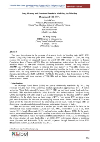
Figure 1. The Returns for VIX-ETFs
4.3 ARFIMA and ARFIMA-FIGARCH models
The next step explains these sudden changes in variances via dummy variables in the ARFIMA
and ARFIMA-FIGARCH models. The results of long memory are summarized in Table 5. Firstly,
the results of the ARFIMA model without sudden changes in panel A illustrated that all series do
not have long memory effect. It clearly indicates that there is no evidence of long memory in
among VIX-ETFs. It implies the return series shows weak-form market efficiency. Furthermore,
the research investigates if there is dual long-term memory in mean return and conditional
variance exists for VIX-ETFs by applying ARFIMA-FIGARCH model.

-6
-4
-2
0
2
4
6
1/04/2011
2/10/2011
3/21/2011
4/26/2011
6/02/2011
7/12/2011
8/16/2011
9/22/2011
10/27/2011
12/02/2011
1/12/2012
2/22/2012
3/29/2012
5/07/2012
6/12/2012
7/19/2012
8/24/2012
10/02/2012
11/08/2012
12/19/2012
1/29/2013
3/08/2013
4/16/2013
5/22/2013
6/27/2013
8/05/2013
9/11/2013
10/17/2013
11/21/2013
12/30/2013
RVIXM
-20
0
20
40
60
80
1/04/2011
2/10/2011
3/21/2011
4/26/2011
6/02/2011
7/12/2011
8/16/2011
9/22/2011
10/27/2011
12/02/2011
1/12/2012
2/22/2012
3/29/2012
5/07/2012
6/12/2012
7/19/2012
8/24/2012
10/02/2012
11/08/2012
12/19/2012
1/29/2013
3/08/2013
4/16/2013
5/22/2013
6/27/2013
8/05/2013
9/11/2013
10/17/2013
11/21/2013
12/30/2013
RVIXY
-3
-2
-1
0
1
2
1/04/2011
2/10/2011
3/21/2011
4/26/2011
6/02/2011
7/12/2011
8/16/2011
9/22/2011
10/27/2011
12/02/2011
1/12/2012
2/22/2012
3/29/2012
5/07/2012
6/12/2012
7/19/2012
8/24/2012
10/02/2012
11/08/2012
12/19/2012
1/29/2013
3/08/2013
4/16/2013
5/22/2013
6/27/2013
8/05/2013
9/11/2013
10/17/2013
11/21/2013
12/30/2013
RSPLV
-20
0
20
40
60
80
100
1/04/2011
2/10/2011
3/21/2011
4/26/2011
6/02/2011
7/12/2011
8/16/2011
9/22/2011
10/27/2011
12/02/2011
1/12/2012
2/22/2012
3/29/2012
5/07/2012
6/12/2012
7/19/2012
8/24/2012
10/02/2012
11/08/2012
12/19/2012
1/29/2013
3/08/2013
4/16/2013
5/22/2013
6/27/2013
8/05/2013
9/11/2013
10/17/2013
11/21/2013
12/30/2013
RUVXY
-30
-20
-10
0
10
1/04/2011
2/10/2011
3/21/2011
4/26/2011
6/02/2011
7/12/2011
8/16/2011
9/22/2011
10/27/2011
12/02/2011
1/12/2012
2/22/2012
3/29/2012
5/07/2012
6/12/2012
7/19/2012
8/24/2012
10/02/2012
11/08/2012
12/19/2012
1/29/2013
3/08/2013
4/16/2013
5/22/2013
6/27/2013
8/05/2013
9/11/2013
10/17/2013
11/21/2013
12/30/2013
RSVXY

Table 5. ARFIMA and ARFIMA-FIGARCH without and with Dummy Variables for Sudden Changes in Variance

VIX-ETF
ARFIMA
ARCH-LM
ARFIMA-FIGARCH
model d-coeff. AIC d-coeff. model d-coeff. AIC
Panel A: Without Dummy Variables for Sudden Changes in Variance
VIXM (1,2)
-0.0319
[0.474]
2.5440
4.5178
[0.0339]*
-0.0122
[0.8190]
(2,3)
0.2096
[0.1589]
2.4619
VIXY (2,2)
0.0061
[0.845]
5.0976
0.0005
[0.9830]
- - - -
SPLV (3,3)
-0.0569
[0.130]
0.6892
14.902
[0.0001]**
-0.0805
[0.0302]*
(2,3)
0.5477
[0.0000]***
0.4291
UVXY (1,0)
-0.034
[0.394]
6.8473 0.0127 - - - -
SVXY (1,0)
-0.0703
[0.248]
4.3673
3.0645e-005
[0.9956]
- - - -
Panel B: With Dummy Variables for Sudden Changes in Variance
VIXM (1,2)
-0.0371
[0.416]
2.5491
4.3442
[0.0375]*
-0.0206
[0.6628]
(2,3)
0.1964
[0.0093]**
2.4662
VIXY (2,2)
0.0060
[0.848]
5.1032
0.0005
[0.9827]
- - - -
SPLV (3,3)
-0.0463
[0.121]
0.7272
16.444
[0.0001]**
-0.1153
[0.0000]***
(2,3)
0.5111
[0.0000]***
0.4430
UVXY (2,1)
-0.9933
[0.000]***
6.8653
0.0270
[0.8695]
- - - -
SVXY (1,0)
-0.0749
[0.231]
4.3760
2.5398e-005
[0.9960]
- - - -
Note: *, ** and *** are significance at 10, 5 and 1% levels, respectively; p-values are in parentheses.

The finding reveals that VIXM does not exhibit long memory or persistence, as d parameter is
statistically insignificant; but SPLV shows long memory or persistence as d parameter is
statistically significant for mean returns while it does for conditional variance.
From an extensive analysis of the ARFIMA model with sudden changes in panel B; the result of
UVXY present that the process is not mean-reverting in the sense that any shock to the process
will displace it from its starting point. We also join the structure breaks in mean return and
conditional variance by ARFIMA-FIGARCH model. The results revealed that VIXM and SPLV
existed long memory, as d parameter is statistically significant. An important implication of this
finding is that considering structure breaks can provide the return series existing in inefficient
market, so one can use past price to predicate their future price for VIXM and SPLV.
This article showed statistically significant results of dual long memory in VIXM and SPLV.
VIXM tracks SP 500 VIX mid-term futures index and SPLV tracks SP 500 low volatility
index but VIXY, UVXY, and SVXY track SP 500 VIX short-term Futures Index. The finding
implies that VIX short-term volatility trend cannot predicate in opposition different period and
pattern. In other words, VIX measure the volatility of the Standard and Poor’s 500 (SP 500) so it
caused VIXpossess weak-form efficiency market in short-term VIX-ETFs.
5. Conclusion
This study investigated sudden shifts of volatility and examined long memory for VIX-ETFs.
The results of ARFIMA model displayed that there was no long memory property in the VIX-ETF
returns, implying the weak-form efficiency market. Next, this study also tested the long memory
property in conditional variance series of VIX-ETFs. The estimation results indicated that
ARFIMAR-FIGARCH with structure breaks model have better exposes long memory property in
conditional variance of return series.
Roughly speaking, the work failed to reject weak-form market efficiency, because the presence
of long memory in the volatility appears, and VIXM and SPLV presented reverting to its mean.
The returns of VIXM and SPLV can be predicted due to the facts that dependence between distant
observations was evident. Thus, fund managers and investors may apply the empirical results by
possessing a position on VIXM and SPLV.

References
Abu-Qarn, A. S. and S. Abu-Bader (2008). Structural Breaks in Military Expenditures: Evidence
for Egypt, Israel, Jordan and Syria. Peace Economics, Peace Science, and Public Policy
14(1): 1-23.
Ackert, L. F. and Y. S. Tian (2008). Arbitrage, Liquidity, and the Valuation of Exchange Traded
Funds. Financial Markets, Institutions and Instruments 17(5): 331-362.
Arouri, M. E., Hammoudeh, S. , Lahian, A. and Nguyen, D.K. (2012). Long Memory and
Structural Breaks in Modeling the Return and Volatility Dynamics of Precious Metals. The
Quarterly Review of Economics and Finance 52(2): 207-218.
Badhani, K. N. (2008). Modeling Aggregate Stock Market Volatility with Structural Breaks in
India. Decision 35(2): 87-107.
Bai, J. and P. Perron (2003). Computation and Analysis of Multiple Structural Change Models.
Journal of Applied Econometrics 18(1): 1-22.
Baillie, R. T., Bollerslev, T., and Mikkelsen, H. O. (1996). Fractionally Integrated Generalized
Autoregressive Conditional Heteroskedasticity. Journal of Econometrics 74(1): 3-30.
Barnhart, S. W. and S. Rosenstein (2010). Exchange-Traded Fund Introductions and Closed-End
Fund Discounts and Volume. Financial Review 45(4): 973-994.
Blitz, D., Huij, J. and Swinkels, L. (2012). The Performance of European Index Funds and
Exchange-Traded Funds. European Financial Management 18(4): 649-662.
Bollerslev, T. (1986). Generalized Autoregressive Conditional Heteroscedasticity. Journal of
Econometrics 31: 307-327.
Bum, S. K. (2011). Linkages between the U.S. and ASIA-Pacific Exchange Traded Funds (ETF)
Markets: Evidence from the 2007-2008 Global Financial Crisis. Asian Academy of
Management Journal of Accounting and Finance 7(1): 52-72.
Caporale, G. M. and L. A. Gil-Alana (2008). Long Memory and Structural Breaks in the Spanish
Stock Market Index. Open Operational Research Journal 2: 13-17.
Cerrato, M., Kim, H., and MacDonald, R. (2013). Equilibrium Exchange Rate Determination and
Multiple Structural Changes. Journal of Empirical Finance 22: 52-66.
Chen, J. H. and J. F. Diaz (2013). Long Memory and Shifts in the Returns Of Green and Non-
Green Exchange-Tranded Funds (ETFs). International Journal of Humanities and Socience
Invenyion 2(10): 29-32.
Choi, Kyongwook, Wei-choun Yu, Eric Zivot (2010). Long Memory versus Structural Breaks in
Modeling and Forecasting Realized Volatility. Journal of International Money and Finance
29(5): 857-875.
Chunxia, Y., X. Bingying, S. Hu, R. Wang (2012). A Study of The Interplay Between The
Structure Variation and Fluctuations of The Shanghai Stock Market. Physica A: Statistical
Mechanics and its Applications 391(11): 3198-3205.
Covarrubias, G., Bradley T. Ewing, Scott E. Hein, and Mark A. (2006). Modeling Volatility
Changes in the 10-year Treasury. Physica A: Statistical Mechanics and Its Applications
369(2): 737-744.
Daigler, R. T., Ann Marie Hibbert, and Ivelina Pavlova (2014). Examining the Return–Volatility
Relation for Foreign Exchange: Evidence from the Euro VIX. Journal of Futures Markets
34(1): 74-92.
Drenovak, M., Uroševic, B. and Jelic, R. (2012). European Bond ETFs-Tracking Errors and
Sovereign Debt Crisis. Working paper, University of Birmingham.
Engle, R. F. (1982). Autoregressive Conditional Heteroscedasticity with Estimates of the
Variance of United Kingdom Inflation. Econometrics Journal 50: 987-1008.
Esteve, V., Manuel Navarro-Ibáñez, and María A. Prats (2013). The Spanish Term Structure of
Interest Rates Revisited: Cointegration with multiple structural breaks, 1974–2010.
International Review of Economics and Finance 25: 24-34.

Ewing, B. T. and F. Malik (2013). Volatility Transmission between Gold and Oil Futures under
Structural Breaks. International Review of Economics and Finance 25: 113-121.
Fama, E. F. (1965). The Behavior of Stock Market Prices. Journal of Business and Economic
Statistics 38(1): 34-105.
Fernandez, V. (2005). Structural Breakpoints in Volatility in International Markets. IIIS
Discussion Paper 76.
Fleming, J., Ostdiek, B. and Whaley, R. E. (1995). Predicting Stock Market Volatility: A New
Measure. Journal of Futures Markets 15(3): 265-302.
Gadea, M., A. Montañés and M. Reyes (2004). The European Union and the US dollar: From
Post-Bretton-Woods to the Euro. Journal of International Money and Finance 23(7-8): 1109-
1136.
Granger, C. W. J. and R. Joyeux (1980). An Introduction to Long-Memory Time Series Models
and Fractional Differencing. Journal of Time Series Analysis 1(1): 15-29.
Guedj, I. and J. C. Huang (2009). Are ETFs Replacing Index Mutual Funds? San Francisco
Meetings Paper. Available at SSRN: http://ssrn.com/abstract=1108728.
Guo, W. and M. E. Wohar (2006). Identifying Regime Changes in Market Volatility. Journal of
Financial Research 29(1): 79-93.
Herzberg, M. and P. Sibbertsen (2004). Pricing of Options under Different Volatility models.
Technical Report / Universität Dortmund, SFB 475 Komplexitätsreduktion in Multivariaten
Datenstrukturen 2004(62).
Hosking, J. R. M. (1981). Fractional Differencing. Biometrika 68(1): 165-176.
Houweling, P. (2012). On the Performance of Fixed-Income Exchange-Traded Funds. The
Journal of Index Investing 3(1): 39-44.
Hughen, J. C. and P. G. Mathew (2009). The Efficiency of International Information Flow:
Evidence from the ETF and CEF prices. International Review of Financial Analysis 18(1–
2): 40-49.
Huskaj, B. (2013). Long Memory in VIX Futures Volatility. Review of Futures Markets 21(1):

33-50.
Inclan, C. and G. C. Tiao (1994). Use of Cumulative Sums of Squares for Retrospective
Detection of Changes of Variance. Journal Of the American Statistical Association 89(427):
913-923.
Ivanov, S. (2012). REIT ETFs Performance During The Financial Crisis. Journal of Finance and
Accountancy 10: 1-9.
Ivanov, S. (2013). The influence of ETFs on The Price Discovery of Gold, Silver and Oil.
Journal of Economics and Finance 37(3): 453-462.
Jares, T. B. and A. M. Lavin (2004). Japan and Hong Kong Exchange-Traded Funds (ETFs):
Discounts, Returns, and Trading Strategies. Journal of Financial Services Research 25(1):
57-69.
Johnson, W. F. (2009). Tracking Errors of Exchange Traded Funds. Journal of Asset
Management 10(4): 253-262.
Jouini, J. and M. Boutahar (2005). Evidence on Structural Changes in U.S. Time Series.
Economic Modelling 22(3): 391-422.
Kang, S. H. and S. M. Yoon (2007). Long Memory Properties in Return and Volatility: Evidence
from the Korean Stock Market. Physica A: Statistical Mechanics and Its Applications
385(2): 591-600.
Kang, S. H., H. G. Cho, and S. M. Yoon (2009). Modeling Sudden Volatility Changes: Evidence
from Japanese and Korean Stock Markets. Physica A: Statistical Mechanics and its
Applications 388(17): 3543-3550.
Krause, T. and Y. Tse (2013). Volatility and Return Spillovers in Canadian and U.S. Industry
ETFs. International Review of Economics and Finance 25: 244-259.

Kumah, F. Y. (2011). A Markov-Switching Approach to Measuring Exchange Market Pressure.
International Journal of Finance and Economics 16(2): 114-130.
Kyongwook, C. and H. Shawkat (2009). Long Memory in Oil and Refined Products Markets.
Energy Journal 30(2): 97-116.
Lin, Ching-Chung, Shih-Ju Chan, Hsinan Hsu (2006). Pricing Efficiency of Exchange Traded
Funds in Taiwan. Journal of Asset Management 7(1): 60-68.
Lixia, Wang, Iftikhar Hussain, and Adnan Ahmed (2010). Gold Exchange Traded Funds: Current
Developments and Future Prospects in China. Asian Social Science 6(7): 119-125.
Mukul, Mukesh Kumar, Vikrant Kumar and Sougata Ray (2012). Gold ETF Performance: A
Comparative Analysis of Monthly Returns. IUP Journal of Financial Risk Management 9(2):
59-63.
Padungsaksawasdi, C. and R. T. Daigler (2013). The Return-Implied Volatility Relation for
Commodity ETFs. Journal of Futures Markets: 1-27.
Pesaran, M. H. and A. Timmermann (2004). How Costly Is It to Ignore Breaks When Forecasting
The Direction of A Time Series? International Journal of Forecasting 20(3): 411-425.
Sadique, S. and P. Silvapulle (2001). Long-Term Memory in Stock Market Returns: International
Evidence. International Journal of Finance and Economics 6(1): 59-67.
Whaley, R. E. (2000). The Investor Fear Gauge. Journal of Portfolio Management 26(3): 12-17.
Wiphatthanananthakul, C. C. and S. Sriboonchitta (2010). ARFIMA-FIGARCH and ARFIMA -
FIAPARCH on Thailand Volatility Index. International Review of Applied Financial Issues
and Economics 2(1): 193-212.
Wong, K. H. Y. and S. Wai Cheong (2010). Exchange-Traded Funds in Bullish and Bearish
Markets. Applied Economics Letters 17(16): 1615-1624.
Zainudin, R. and R. S. Shaharudin (2011). An Investigation of Structural Breaks on Spot and
Futures Crude Palm Oil Returns. Journal of Applied Sciences Research 7(9): 1872-1885.
Zhu, B. and Y. Wei (2013). Carbon Price Forecasting with A Novel Hybrid ARIMA and Least
Squares Support Vector Machines Methodology. Omega 41(3): 517-524.

Modelling Volatility Dynamics of VIX-ETFs with Structural Breaks and Long Memory

Recommandé

Recommandé

Contenu connexe

Tendances

Tendances (7)

Similaire à Modelling Volatility Dynamics of VIX-ETFs with Structural Breaks and Long Memory

Similaire à Modelling Volatility Dynamics of VIX-ETFs with Structural Breaks and Long Memory (20)

Plus de KLIBEL

Plus de KLIBEL (20)

Dernier

Dernier (20)

Modelling Volatility Dynamics of VIX-ETFs with Structural Breaks and Long Memory