2. Iterative Method
Simultaneous linear algebraic equation occur in various fields of Science
and Engineering.
We know that a given system of linear equation can be solved by
applying Gauss Elimination Method and Gauss – Jordon Method.
But these method is sensitive to round off error.
In certain cases iterative method is used.
Iterative methods are those in which the solution is got by successive
approximation.
Thus in an indirect method or iterative method, the amount of
computation depends on the degree of accuracy required.
2
Introduction:
3. Iterative Method
Iterative methods such as the Gauss – Seidal method give the user
control of the round off.
But this method of iteration is not applicable to all systems of equation.
In order that the iteration may succeed, each equation of the system
must contain one large co-efficient.
The large co-efficient must be attached to a different unknown in that
equation.
This requirement will be got when the large coefficients are along the
leading diagonal of the coefficient matrix.
When the equation are in this form, they are solvable by the method of
successive approximation.
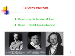
Two iterative method - i) Gauss - Jacobi iteration method
ii) Gauss - Seidal iteration method
3
Introduction (continued..)
4. Gauss – Jacobi Iteration Method:
The first iterative technique is called the Jacobi method named after
Carl Gustav Jacob Jacobi(1804- 1851).
Two assumption made on Jacobi method:
1)The system given by
4
a x a x a x
b
- - - - - - - - (1)
11 1 12 2 1 n n
1
a x a x a x
b
n n
21 1 22 2 2 2
a x a x a x
b
n 1 1 n 2 2
nn n n
- - - - - - - - (2)
- - - - - - - - (3)
has a unique solution.
5. Gauss – Jacobi Iteration Method
5
Second assumption:
3 7 13 76 1 2 3 x x x
5 3 28 1 2 3 x x x
12 3 0 1 1 2 3 x x x
12 3 0 1 1 2 3 x x x
5 3 28 1 2 3 x x x
3 7 13 76 1 2 3 x x x
7. To begin the Jacobi method ,solve
7
Gauss– Jacobi Iteration Method
a x a x a x
b
n n
11 1 12 2 1 1
a x a x a x
b
n n
21 1 22 2 2 2
a x a x a x
b
n 1 1 n 2 2
nn n n
12. Gauss– Jacobi Iteration Method
12
a x a x a x
b
- - - -(1)
11 1 12 2 1 n n
1
a x a x a x
b
n n
21 1 22 2 2 2
a x a x a x
b
n 1 1 n 2 2
nn n n
- - - -(2)
- - - -(3)
16. Gauss– Jacobi Iteration Method
Solution:
In the given equation , the largest co-efficient is attached to a
different unknown.
Checking the system is diagonally dominant .
Here
Then system of equation is diagonally dominant .so iteration method
can be applied.
16
27 27 6 1 7 11 12 13 a a a
17. Gauss– Jacobi Iteration Method
From the given equation we have
17
85 6 2 3
27
1
x x
x
72 6 2 1 3
15
2
x x
x
110 1 2
54
3
x x
x
(1)
22. Gauss –Seidal Iteration Method
Modification of Gauss- Jacobi method,
named after Carl Friedrich Gauss and Philipp Ludwig Von Seidal.
This method requires fewer iteration to produce the same degree
of accuracy.
This method is almost identical with Gauss –Jacobi method except
in considering the iteration equations.
The sufficient condition for convergence in the Gauss –Seidal
method is that the system of equation must be strictly diagonally
dominant
22
23. Gauss –Seidal Iteration Method
Consider a system of strictly diagonally dominant equation as
23
a x a x a x
b
n n
11 1 12 2 1 1
a x a x a x
b
n n
21 1 22 2 2 2
a x a x a x
b
n 1 1 n 2 2
nn n n
- - - - -(1)
- - - - - (2)
- - - - - (3)
26. Gauss –Seidal Iteration Method
26
The successive iteration are generated by the scheme called
iteration formulae of Gauss –Seidal method are as
The number of iterations k required depends upon the desired
degree of accuracy
27. Gauss –Seidal Iteration Method
Soln: From the given equation ,we have
- - - - - - - (1)
- - - - - - -(2)
- - - - - - - (3)
27
85 6 2 3
27
1
x x
x
72 6 2 1 3
15
2
x x
x
110 1 2
54
3
x x
x
29. Gauss –Seidal Iteration Method
1st Iteration:
29
1.91317
(1)
(1)
(1)
3
3.54074
2
3.14815
1
x
x
x
30. Gauss –Seidal Iteration Method
30
For the second iteration,
1.91317
(1)
(1)
(1)
3
3.54074
2
3.14815
1
x
x
x
2.43218
(1)
(2)
27
85 6
(1)
3
2
1
x x
x
3.57204
(2)
72 6 2
(2)
15
(1)
3
1
2
x x
x
1.92585
(2)
(2)
54
110
(2)
2
1
3
x x
x
31. Gauss –Seidal Iteration Method
Thus the iteration is continued .The results are tabulated.
S.No Iteration or
approximation
x i ( , ,2,3..)
x i i i x i ( i
i , ,2,3..)
1 0 0 0 0
2 1 3.14815 3.54074 1.91317
3 2 2.43218 3.57204 1.92585
4 3 2.42569 3.57294 1.92595
5 4 2.42549 3.57301 1.92595
6 5 2.42548 3.57301 1.92595
31
(i i, ,2,3..)
1,
2
3
4th and 5th iteration are practically the same to four places.
So we stop iteration process.
Ans: x x x
1.9260
3
3.57301;
2
2.4255;
1
32. Gauss –Seidal Iteration Method
Comparison of Gauss elimination and Gauss- Seidal Iteration methods:
Gauss- Seidal iteration method converges only for special systems of
equations. For some systems, elimination is the only course
available.
The round off error is smaller in iteration methods.
Iteration is a self correcting method
32