1. Complex Numbers, Vectors and Co-ordinates:
Getting the Best from the HP-35s.
Introduction
In the third quarter of 2007, Hewlett Packard introduced the HP-35s pocket calculator. The model
number (HP-35) commemorates 35 years since the introduction of their first pocket calculator,
the HP-35A, thirty-five years before (1972). The HP-35A revolutionized computing and set an
exceptionally high standard of quality and performance.
The new HP-35s may not have the same general impact as its famous forebear, but some of its
features and approaches to work methodologies will cause some concern for users in the
surveying community. This is because the method of dealing with co-ordinates and their
connection with azimuths and distances is very different in the HP-35s. The Rectangular to Polar
(and vice versa) functions no longer appear on the calculator, for example, and complex numbers
are almost completely integrated with regular real-number calculator operations.
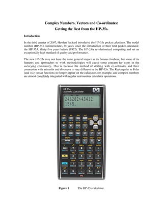
Figure 1 The HP-35s calculator.

2. Comparisons with Other HP Calculators
The HP-33S calculator, released in 2004, followed a long line of mid-range pocket calculators
with broad functionality, starting with the HP-25, released in the late 1970s1. These calculators
had all the computing power of the upper-range machines, but lacked the expansion, alphabetical,
graphing and some high-end calculation capabilities of the more expensive calculators (e.g., HP-
41, HP-48). For general number crunching, however, they were excellent. This line of calculators
was a very popular choice for surveyors, especially for personal and field calculators.
With these calculators, the process of working with a traverse, for example, was consistent across
the machines and the years. The azimuth and distance of each line in the traverse were entered in
the appropriate format and arrangement, they were converted to latitude and departure
components (using Polar to Rectangular conversion), and these were added in the statistical
registers. The resulting sums of the latitudes and departures could be converted back to a closing
azimuth and distance using the Rectangular to Polar conversion).
The HP-50g calculator is currently HP’s top-end offering, with formidable computational power.
It is a machine that essentially runs the HP-48GX’s operating system and software, with
extensions and developments, on a new hardware platform. While the operating system has
changed dramatically from the first HP high-end pocket calculator, the HP-50g can trace its roots
back to that machine, the venerable HP-65.
With the HP-48 onwards (the HP-48, HP-49 and HP-50 models), the operating system is
completely object-oriented, which is noticeable in how the calculator works. The method of
working with a traverse with these calculators is to enter the distance and azimuth as a vector.
Subsequent vectors can be added to this vector. The vector can be viewed in rectangular mode,
showing co-ordinates, or in polar mode, showing the azimuth and distance of the vector. The
calculator includes tools for building, decomposing and manipulating vectors, which make
handing these relatively simple.
The HP-35s is part-way between the approaches of the HP-33S and the HP-50g. It allows the use
of vectors, but only in a very limited way. Co-ordinates and vectors in 2-D are better represented
as complex numbers, and the calculator has limited tools to work with these in ways that are
useful for surveyors. There is no simple way to work traverse measurements in the same manner
as with the HP-33S, but there are insufficient tools to allow work to be done in the same manner
as in the HP-50g.
In summary, in order to work with traverse sides and co-ordinates in the HP-35s, you need to
know about complex numbers, vectors and how these all relate to each other, at least in the
context of how the HP-35s works. This is not to say that the approach taken in the HP-35s is
wrong, merely different from how things were done in the past.
This document is intended to inform surveyors and surveying students about things that are handy
to know about complex numbers, vectors and co-ordinates, as they apply to how things are done
with the HP-35s. Once the users can get the ideas into their way of thinking, it should be much
easier to get the calculator to do what you need it to do.
1
It could be argued that the line really begins with the HP-45, released around 1973, but the HP-45 lacked
programmability. The HP-55 of the same era had some programming capacity, but was not as popular as
the other calculators in the HP model line at that time.

3. Real and Other Numbers and the Argand Plane
All the numbers we tend to run across in everyday life are real numbers. Real numbers include
the integers, fractions, decimal numbers, irrational numbers such as 2 , and transcendental
numbers, such as π. Real numbers can be represented on a number line. However, there are some
algebraic equations that cannot be solved in terms of real numbers, e.g., x2 + 4x + 6 = 0, which
has the solutions x = –2 + (−2) and –2 – (−2) . Square roots of negative numbers are not
defined among the real numbers to allow these solutions.
A solution to this difficulty was the creation of imaginary numbers, all of which are able to be
expressed as a i, where a is any real number and i is the square root of –1. Since imaginary
numbers are simply the value i scaled by a real number, the imaginary numbers can be
represented on an imaginary number line.
If we have to deal with a single number such as one of those above, e.g., x = –2 + (−2) , this is
often expressed as x = –2 + i 2 , which is made up of two parts, one real (–2) and one imaginary
i 2 . This type of number is termed a complex number, as it is made up of more than one
number, and cannot be reduced to anything simpler than this two-part number.
Figure 2 The Argand Plane, used for locating complex numbers.
If the real part of the number can be represented on the real number line, while the imaginary part
can be represented on the imaginary number line, it is possible to represent the complex number
on a 2-D plane having co-ordinates on each number line, with the two number lines at right
angles. This plane is known as the Argand Plane, and the representation of the complex number
x = –2 + i 2 is shown in Figure 2.
The –2 value is located on the real number axis (designated with the letter ℜ for ‘real’), and the
i 2 value is located on the imaginary number axis (designated with the letter ℑ for

4. ‘imaginary’). The point produced from these two co-ordinates is the location of the complex
number x in the Argand Plane.
The complex number x can also be located using polar co-ordinates, rather than rectangular co-
ordinates. In this case, the distance of the point x from the origin of the Argand Plane (r) and the
rotation (θ) of the line between the origin and the point x, taken counter-clockwise from the
positive real axis, define the same line. In the case of the complex number x, the value of r is
2.4495 and the angle is 144°.7356, so x can be expressed as –2 + i 2 or 2.4495 θ 144°.7356.
Both representations are equivalent and the choice between them comes down to convenience at
any given time. In many cases in mathematics, the angle is recorded in radians, rather than
degrees, but this is a straightforward difference, and converting decimal degrees to radians and
vice versa are built-in functions..
The Argand plane follows the conventions of mathematical co-ordinate representations, in that all
rotations are measured counter-clockwise from the horizontal axis extending to the right. In the
surveying and mapping disciplines, a different convention applies, so we have to think about a
‘Surveying Argand Plane’ to work with co-ordinates in the surveying sense. This is shown in
Figure 3.
Figure 3 The ‘Surveying Argand Plane,’ showing a point with both rectangular and polar
co-ordinates.
In this case, the real axis is up the page, and is equivalent to the usual North or Y axis, while the
imaginary is to the right, equivalent to the usual East or X axis. A point with the co-ordinates East
= 5, North = –6 has been shown. The equivalent polar co-ordinates are r = 7.8105 and θ =
140°.1944.
Of course, the same point could be designated as z = –6 + 5i, or z = 7.8102 θ 144°.1944, or z =
7.8102 θ 2.4469 radians.

5. So there are many ways to represent a complex number, and a complex number can be used to
represent a point in a 2-D space.
In the same way that a complex number can be represented in both rectangular and polar forms, a
vector can be represented in both forms. In polar form, it is the familiar azimuth and distance of a
line. In rectangular form, the vector appears as orthogonal components, usually the latitude and
departure of the line. In fact, in the HP-35s, it is more useful to represent 2-D vectors as complex
numbers than as actual vectors.
Working with the HP-35s
The HP-35s allows complex numbers to be carried through many calculations, registers and stack
locations in the same manner as conventional real numbers. The calculator allocates sufficient
memory for the full 12-digit precision of both components of the complex number to be
maintained. If the display is too small to show the full precision, the number can be scrolled to the
left or right to allow the user to see the full precision of the complex number’s components.
With this complex number capability, combined with the lack of built-in ways of working with
vectors solely by components (which was the way it was done on the HP-33s back to the HP-45),
it is sensible to work completely with the complex number representations, rather than trying to
deal with the components manually. It also allows some of the capabilities of the HP-50g to be
used for work on the HP-35s.
Displaying Complex Numbers
The HP-35s can display complex numbers in two forms when in RPN mode. These are the
rectangular and polar forms. The DISPLAY menu controls which is used for display (note that
the internal representation remains the same; only the display is changed). Pressing the gold (left)
key, followed by the < cursor key (DISPLAY) will show the DISPLAY menu. Scrolling down
will show options 9 and 10. These can be selected by scrolling to the appropriate value and
pressing enter, or by pressing the number on the keyboard (use .0 for 10). Option 9 sets the
calculator to display complex numbers in x i y mode (rectangular), while option 10 sets the
calculator to display complex numbers in r θ α mode (polar).
Regardless of the complex number was entered, the display mode will change how all complex
numbers are displayed. Complex numbers may be entered in either mode, regardless of the
current display more.
Note that when complex numbers are displayed in r θ α mode, there is no space between the
characters, so the real component ends right next to the displayed θ, which is right next to the
imaginary part. It is very easy to read the θ as the digit 8, e.g., 123.4567θ987.6543.
Entering Co-ordinates as a Complex Number
In many cases, co-ordinates are used in conjunction with vector calculations, and so they are most
useful when already in the calculator’s complex number form. To enter a co-ordinate pair as a
complex number, key in the Northing or Y value first, press the i key (fourth from the left on the
second row from the top), then key in the Easting or X value. If you press the Enter key, the
complex number will be duplicated into the Y stack register, and will appear twice, once in each
line of the display.

6. If a second co-ordinate pair is entered, it is possible to subtract one from the other, which will
produce a complex number whose components are the differences in Northings and Eastings, if
the display setting is for rectangular mode. Changing the display mode to viewing complex
numbers in polar form, the complex number appears as a vector, with distance and orientation
displayed.
When entering co-ordinates, remember the order: North, then i, then East.
To enter the co-ordinate as part of a program, move the Northing value to the Y register (line 1)
and the Easting value to the X register (line 2). This can be done with two RCL statements. Then
enter 0 i 1 on the next line of the program, then ×, then +. This multiplies the Easting value by i,
forming a complex number with the value 0 i Easting. Adding the Northing as a real number
makes the complex number Northing i Easting, which is now ready for further processing. This
approach can be seen in several of the programs, and as it takes three program lines beyond
recalling the co-ordinates, it isn’t worth having a separate program for this operation.
Entering Vectors as a Complex Number
Vectors can be entered as a distance and azimuth, providing the polar form of a complex number.
Because an angle is involved, it is necessary to enter the angular part in the same form as the
current calculator setting. For most surveying work, this will be degrees, but it is also possible to
use radians. To enter the vector, key in the distance, then press the blue (right) arrow key,
followed by the θ key (on the lower face of the i key), then the azimuth in decimal degrees.
Once the Enter key is pressed, the complex number will be pushed up the stack, and will be
displayed in the current mode.
If two vectors have been entered, the vector sum can be obtained by having the two vectors on the
stack and pressing the + key. If the calculator is on polar display mode, this is the same as keying
in the azimuth and distance of each line, converting it to rectangular components, adding the
components (usually in the statistical registers), retrieving the sums and converting them back to
polar representation; but in this case it can be done with a single keystroke.
One complication is the issue of entering an azimuth in degrees, minutes and seconds. The
azimuth must be converted to decimal degrees, but this cannot be done within the complex
number, nor within the complex number entry mode. (This can be done on the HP-50g, as vectors
may be built directly from elements on the stack.)
The solution is a small program that allows the user to enter azimuths in degrees, minutes and
seconds, followed by the distance, and convert them to a complex number. The program (Utility
3) will accomplish this. The azimuth is entered in HP notation (DDD.MMSSsss).
Extracting the Azimuth and Distance from a Complex Number
First make sure the calculator is in DEGREES mode. If the complex number is in the X register,
press the blue right-arrow key, then ABS. This is the distance. Before doing anything else, press
the blue right arrow key and then LASTx, to bring the complex number back to the X register.
Press the gold left arrow key, then ARG. The value in line 2 (the X register) is the azimuth in
decimal degrees. If this value is negative, enter 360, then press +. Press the blue right arrow key
and →HMS to convert the azimuth to degrees, minutes and seconds (in HP notation).

7. The calculator now has the distance in the Y register (line 1) and the azimuth in HP notation in
the X register (line 2).
Extracting Co-ordinates from a Complex Number
In the HP-35s, there is no built-in function to extract the real or imaginary parts from a complex
number. This means that if the co-ordinates of a point, or the latitude and departure of a line, are
required for separate processing, they have to be extracted from the complex number by several
steps. A simple program to do this is available (Utility 4).
Other Capabilities
The HP-35s can do a number of other operations with complex numbers. as well as addition and
subtraction, two complex numbers can be multiplied together, or one may be divided into the
other. Complex numbers may be raised to powers, and these powers may also be complex
numbers. Complex numbers can be used as the exponent of e, and natural logarithms of complex
numbers may also be calculated. Trigonometric functions can also use complex numbers as
arguments. As already covered, the absolute value (distance or length) and argument (orientation
or angle) of a complex number may be calculated.
Multiplication, division and exponentiation as complex numbers are not very relevant to everyday
vector usage, and so may be ignored by most surveying people, together with logarithms, anti-
logarithms and trigonometric functions involving complex numbers.
Two Other Programs
Two other programs are supplied to cover two small areas of deficiency in the HP-35s calculator.
These two deficiencies are the absence of functions that can directly add and subtract angles in
degrees, minutes and seconds. These two functions are extremely handy when working with
traverses and angle observations, and while present in the HP-50g, are not present in the HP-35s,
nor in the HP-33s.
The HMS+ program is Utility 1, while HMS– is Utility 2. These programs are assigned to the C
and D keys as they are extremely useful for many surveying calculations.
Note that all these programs can be called as sub-routines from inside other programs, to
accomplish tasks required by those programs. While the programs will affect values on the stack,
they are designed to avoid causing problems with values in the storage registers that are
designated by letters, i.e., A to Z.
Dr. Bill Hazelton
17th October, 2007.