An antiderivative of a function is a function whose derivative is the given function. The problem of antidifferentiation is interesting, complicated, and useful, especially when discussing motion.

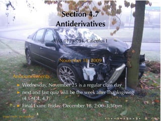
1. Section 4.7
Antiderivatives
V63.0121.034, Calculus I
November 18, 2009
Announcements
Wednesday, November 25 is a regular class day
next and last quiz will be the week after Thanksgiving
(4.1–4.4, 4.7)
Final Exam: Friday, December 18, 2:00–3:50pm
. .
Image credit: Ian Hampton
. . . . . .

2. Why the MVT is the MITC
Most Important Theorem In Calculus!
Theorem
Let f′ = 0 on an interval (a, b). Then f is constant on (a, b).
Proof.
Pick any points x and y in (a, b) with x < y. Then f is continuous
on [x, y] and differentiable on (x, y). By MVT there exists a point
z in (x, y) such that
f(y) − f(x)
= f′ (z) = 0.
y−x
So f(y) = f(x). Since this is true for all x and y in (a, b), then f is
constant.
. . . . . .

3. Theorem
Suppose f and g are two differentiable functions on (a, b) with
f′ = g′ . Then f and g differ by a constant. That is, there exists a
constant C such that f(x) = g(x) + C.
Proof.
Let h(x) = f(x) − g(x)
Then h′ (x) = f′ (x) − g′ (x) = 0 on (a, b)
So h(x) = C, a constant
This means f(x) − g(x) = C on (a, b)
. . . . . .

4. Objectives
Given an expression for
function f, find a
differentiable function F
such that F′ = f (F is
called an antiderivative
for f).
Given the graph of a
function f, find a
differentiable function F
such that F′ = f
Use antiderivatives to
solve problems in
rectilinear motion
. . . . . .

5. Hard problem, easy check
Example
Find an antiderivative for f(x) = ln x.
. . . . . .

6. Hard problem, easy check
Example
Find an antiderivative for f(x) = ln x.
Solution
???
. . . . . .

7. Hard problem, easy check
Example
Find an antiderivative for f(x) = ln x.
Solution
???
Example
is F(x) = x ln x − x an antiderivative for f(x) = ln x?
. . . . . .

8. Hard problem, easy check
Example
Find an antiderivative for f(x) = ln x.
Solution
???
Example
is F(x) = x ln x − x an antiderivative for f(x) = ln x?
Solution
d 1
(x ln x − x) = 1 · ln x + x · − 1
dx x
= ln x
. . . . . .

9. Hard problem, easy check
Example
Find an antiderivative for f(x) = ln x.
Solution
???
Example
is F(x) = x ln x − x an antiderivative for f(x) = ln x?
Solution
d 1
(x ln x − x) = 1 · ln x + x · − 1
dx x
= ln x
Yes!
. . . . . .

10. Outline
Tabulating Antiderivatives
Power functions
Combinations
Exponential functions
Trigonometric functions
Finding Antiderivatives Graphically
Rectilinear motion
. . . . . .

11. Antiderivatives of power functions
Recall that the derivative of a power function is a power function.
Fact
The Power Rule If f(x) = xr , then f′ (x) = rxr−1 .
. . . . . .

12. Antiderivatives of power functions
Recall that the derivative of a power function is a power function.
Fact
The Power Rule If f(x) = xr , then f′ (x) = rxr−1 .
So in looking for antiderivatives of power functions, try power
functions!
. . . . . .

13. Example
Find an antiderivative for the function f(x) = x3 .
. . . . . .

14. Example
Find an antiderivative for the function f(x) = x3 .
Solution
Try a power function F(x) = axr
. . . . . .

15. Example
Find an antiderivative for the function f(x) = x3 .
Solution
Try a power function F(x) = axr
Then F′ (x) = arxr−1 , and we want this to be equal to x3 .
. . . . . .

16. Example
Find an antiderivative for the function f(x) = x3 .
Solution
Try a power function F(x) = axr
Then F′ (x) = arxr−1 , and we want this to be equal to x3 .
1
Apparently, r − 1 = 3 =⇒ r = 4, and ar = 1 =⇒ a = .
4
. . . . . .

17. Example
Find an antiderivative for the function f(x) = x3 .
Solution
Try a power function F(x) = axr
Then F′ (x) = arxr−1 , and we want this to be equal to x3 .
1
Apparently, r − 1 = 3 =⇒ r = 4, and ar = 1 =⇒ a = .
4
1 4
So F(x) = x is an antiderivative.
4
. . . . . .

18. Example
Find an antiderivative for the function f(x) = x3 .
Solution
Try a power function F(x) = axr
Then F′ (x) = arxr−1 , and we want this to be equal to x3 .
1
Apparently, r − 1 = 3 =⇒ r = 4, and ar = 1 =⇒ a = .
4
1 4
So F(x) = x is an antiderivative.
4
Check: ( )
d 1 4 1
x = 4 · x 4 −1 = x 3
dx 4 4
. . . . . .

19. Example
Find an antiderivative for the function f(x) = x3 .
Solution
Try a power function F(x) = axr
Then F′ (x) = arxr−1 , and we want this to be equal to x3 .
1
Apparently, r − 1 = 3 =⇒ r = 4, and ar = 1 =⇒ a = .
4
1 4
So F(x) = x is an antiderivative.
4
Check: ( )
d 1 4 1
x = 4 · x 4 −1 = x 3
dx 4 4
Any others?
. . . . . .

20. Example
Find an antiderivative for the function f(x) = x3 .
Solution
Try a power function F(x) = axr
Then F′ (x) = arxr−1 , and we want this to be equal to x3 .
1
Apparently, r − 1 = 3 =⇒ r = 4, and ar = 1 =⇒ a = .
4
1 4
So F(x) = x is an antiderivative.
4
Check: ( )
d 1 4 1
x = 4 · x 4 −1 = x 3
dx 4 4
1 4
Any others? Yes, F(x) = x + C is the most general form.
4
. . . . . .

21. Fact (The Power Rule for antiderivatives)
If f(x) = xr , then
1 r+1
F(x) = x
r+1
is an antiderivative for f…
. . . . . .

22. Fact (The Power Rule for antiderivatives)
If f(x) = xr , then
1 r+1
F(x) = x
r+1
is an antiderivative for f as long as r ̸= −1.
. . . . . .

23. Fact (The Power Rule for antiderivatives)
If f(x) = xr , then
1 r+1
F(x) = x
r+1
is an antiderivative for f as long as r ̸= −1.
Fact
1
If f(x) = x−1 = , then
x
F(x) = ln |x| + C
is an antiderivative for f.
. . . . . .

24. What’s with the absolute value?
F(x) = ln |x| has domain all nonzero numbers, while ln x is
only defined on positive numbers.
. . . . . .

25. What’s with the absolute value?
F(x) = ln |x| has domain all nonzero numbers, while ln x is
only defined on positive numbers.
For positive numbers x,
d d
ln |x| = ln x
dx dx
(which we knew)
. . . . . .

26. What’s with the absolute value?
F(x) = ln |x| has domain all nonzero numbers, while ln x is
only defined on positive numbers.
For positive numbers x,
d d
ln |x| = ln x
dx dx
(which we knew)
For negative numbers
d d 1 1
ln |x| = ln(−x) = · (−1) =
dx dx −x x
. . . . . .

27. What’s with the absolute value?
F(x) = ln |x| has domain all nonzero numbers, while ln x is
only defined on positive numbers.
For positive numbers x,
d d
ln |x| = ln x
dx dx
(which we knew)
For negative numbers
d d 1 1
ln |x| = ln(−x) = · (−1) =
dx dx −x x
We prefer the antiderivative with the larger domain.
. . . . . .

28. Graph of ln |x|
y
.
. f
. (x ) = 1 /x
x
.
. . . . . .

29. Graph of ln |x|
y
.
. (x) = ln |x|
F
. f
. (x ) = 1 /x
x
.
. . . . . .

30. Graph of ln |x|
y
.
. (x) = ln |x|
F
. f
. (x ) = 1 /x
x
.
. (x) = ln |x|
F
. . . . . .

31. Combinations of antiderivatives
Fact (Sum and Constant Multiple Rule for Antiderivatives)
If F is an antiderivative of f and G is an antiderivative of g,
then F + G is an antiderivative of f + g.
If F is an antiderivative of f and c is a constant, then cF is an
antiderivative of cf.
. . . . . .

32. Combinations of antiderivatives
Fact (Sum and Constant Multiple Rule for Antiderivatives)
If F is an antiderivative of f and G is an antiderivative of g,
then F + G is an antiderivative of f + g.
If F is an antiderivative of f and c is a constant, then cF is an
antiderivative of cf.
Proof.
These follow from the sum and constant multiple rule for
derivatives:
If F′ = f and G′ = g, then
(F + G)′ = F′ + G′ = f + g
Again, if F′ = f,
(cF)′ = cF′ = cf
. . . . . .

33. Example
Find an antiderivative for f(x) = 16x + 5
. . . . . .

34. Example
Find an antiderivative for f(x) = 16x + 5
Solution
The expression 8x2 is an antiderivative for 16x, and 5x is an
antiderivative for 5. So
F(x) = 8x2 + 5x + C
is the antiderivative of f.
. . . . . .

35. Exponential Functions
Fact
If f(x) = ax , f′ (x) = (ln a)ax .
. . . . . .

36. Exponential Functions
Fact
If f(x) = ax , f′ (x) = (ln a)ax .
Accordingly,
Fact
1 x
If f(x) = ax , then F(x) = a + C is the antiderivative of f.
ln a
. . . . . .

37. Exponential Functions
Fact
If f(x) = ax , f′ (x) = (ln a)ax .
Accordingly,
Fact
1 x
If f(x) = ax , then F(x) = a + C is the antiderivative of f.
ln a
Proof.
Check it yourself.
. . . . . .

38. Exponential Functions
Fact
If f(x) = ax , f′ (x) = (ln a)ax .
Accordingly,
Fact
1 x
If f(x) = ax , then F(x) = a + C is the antiderivative of f.
ln a
Proof.
Check it yourself.
In particular,
Fact
If f(x) = ex , then F(x) = ex + C is the antiderivative of F.
. . . . . .

39. Logarithmic functions?
Remember we found
F(x) = x ln x − x
is an antiderivative of f(x) = ln x.
. . . . . .

40. Logarithmic functions?
Remember we found
F(x) = x ln x − x
is an antiderivative of f(x) = ln x.
This is not obvious. See Calc II for the full story.
. . . . . .

41. Logarithmic functions?
Remember we found
F(x) = x ln x − x
is an antiderivative of f(x) = ln x.
This is not obvious. See Calc II for the full story.
ln x
However, using the fact that loga x = , we get that
ln a
1
F(x) = (x ln x − x) + C
ln a
is the antiderivative of f(x) = loga (x).
. . . . . .

42. Trigonometric functions
Fact
d d
sin x = cos x cos x = − sin x
dx dx
. . . . . .

43. Trigonometric functions
Fact
d d
sin x = cos x cos x = − sin x
dx dx
So to turn these around,
Fact
The function F(x) = − cos x + C is the antiderivative of
f(x) = sin x.
. . . . . .

44. Trigonometric functions
Fact
d d
sin x = cos x cos x = − sin x
dx dx
So to turn these around,
Fact
The function F(x) = − cos x + C is the antiderivative of
f(x) = sin x.
The function F(x) = sin x + C is the antiderivative of
f(x) = cos x.
. . . . . .

45. Outline
Tabulating Antiderivatives
Power functions
Combinations
Exponential functions
Trigonometric functions
Finding Antiderivatives Graphically
Rectilinear motion
. . . . . .

46. Problem
Below is the graph of a function f. Draw the graph of an
antiderivative for F.
y
.
.
. . . = f(x)
y
. . . . . . .
x
.
1
. 2
. 3
. 4
. 5
. 6
.
.
. . . . . .

47. Using f to make a sign chart for F
Assuming F′ = f, we can make a sign chart for f and f′ to find the
intervals of monotonicity and concavity for for F:
′
. . . . . . .. = F
f
y
. 1
. 2
. 3
. 4
. 5
. 6F
..
.
. .
. . . . . . .
x
.
1 2 3 4 5 6
. . . . . .
.
. . . . . .

48. Using f to make a sign chart for F
Assuming F′ = f, we can make a sign chart for f and f′ to find the
intervals of monotonicity and concavity for for F:
′
. .. .
+ . . . .. = F
f
y
. 1
. 2
. 3
. 4
. 5
. 6F
..
.
. .
. . . . . . .
x
.
1 2 3 4 5 6
. . . . . .
.
. . . . . .

49. Using f to make a sign chart for F
Assuming F′ = f, we can make a sign chart for f and f′ to find the
intervals of monotonicity and concavity for for F:
′
. .. .. .
+ + . . .. = F
f
y
. 1
. 2
. 3
. 4
. 5
. 6F
..
.
. .
. . . . . . .
x
.
1 2 3 4 5 6
. . . . . .
.
. . . . . .

50. Using f to make a sign chart for F
Assuming F′ = f, we can make a sign chart for f and f′ to find the
intervals of monotonicity and concavity for for F:
+ + − ′
. .. .. .. . . .. = F
f
y
. 1
. 2
. 3
. 4
. 5
. 6F
..
.
. .
. . . . . . .
x
.
1 2 3 4 5 6
. . . . . .
.
. . . . . .

51. Using f to make a sign chart for F
Assuming F′ = f, we can make a sign chart for f and f′ to find the
intervals of monotonicity and concavity for for F:
+ + − − ′
. .. .. .. .. . .. = F
f
y
. 1
. 2
. 3
. 4
. 5
. 6F
..
.
. .
. . . . . . .
x
.
1 2 3 4 5 6
. . . . . .
.
. . . . . .

52. Using f to make a sign chart for F
Assuming F′ = f, we can make a sign chart for f and f′ to find the
intervals of monotonicity and concavity for for F:
+ + − − + f ′
. . . . . . . . . . . .. = F
y
. 1
. 2
. 3
. 4
. 5
. 6F
..
.
. .
. . . . . . .
x
.
1 2 3 4 5 6
. . . . . .
.
. . . . . .

53. Using f to make a sign chart for F
Assuming F′ = f, we can make a sign chart for f and f′ to find the
intervals of monotonicity and concavity for for F:
+ + − − + f ′
. . . . . . . . . . . .. = F
y
. 1↗2
. . . 3
. 4
. 5
. 6F
..
.
. .
. . . . . . .
x
.
1 2 3 4 5 6
. . . . . .
.
. . . . . .

54. Using f to make a sign chart for F
Assuming F′ = f, we can make a sign chart for f and f′ to find the
intervals of monotonicity and concavity for for F:
+ + − − + f ′
. . . . . . . . . . . .. = F
y
. 1↗2↗3
. . . . . 4
. 5
. 6F
..
.
. .
. . . . . . .
x
.
1 2 3 4 5 6
. . . . . .
.
. . . . . .

55. Using f to make a sign chart for F
Assuming F′ = f, we can make a sign chart for f and f′ to find the
intervals of monotonicity and concavity for for F:
+ + − − + f ′
. . . . . . . . . . . .. = F
y
. 1↗2↗3↘4
. . . . . . . 5
. 6F
..
.
. .
. . . . . . .
x
.
1 2 3 4 5 6
. . . . . .
.
. . . . . .

56. Using f to make a sign chart for F
Assuming F′ = f, we can make a sign chart for f and f′ to find the
intervals of monotonicity and concavity for for F:
+ + − − + f ′
. . . . . . . . . . . .. = F
y
. 1↗2↗3↘4↘5
. . . . . . . . . 6F
..
.
. .
. . . . . . .
x
.
1 2 3 4 5 6
. . . . . .
.
. . . . . .

57. Using f to make a sign chart for F
Assuming F′ = f, we can make a sign chart for f and f′ to find the
intervals of monotonicity and concavity for for F:
+ + − − + f ′
. . . . . . . . . . . .. = F
y
. 1 ↗ 2 ↗ 3 ↘ 4 ↘ 5 ↗ 6F
. . . . . . . . . . ..
.
. .
. . . . . . .
x
.
1 2 3 4 5 6
. . . . . .
.
. . . . . .

58. Using f to make a sign chart for F
Assuming F′ = f, we can make a sign chart for f and f′ to find the
intervals of monotonicity and concavity for for F:
+ + − − + f ′
. . . . . . . . . . . .. = F
y
. 1 ↗ 2 ↗ 3 ↘ 4 ↘ 5 ↗ 6F
. . .. . . . . . . . . .
max
.
. .
. . . . . . .
x
.
1 2 3 4 5 6
. . . . . .
.
. . . . . .

59. Using f to make a sign chart for F
Assuming F′ = f, we can make a sign chart for f and f′ to find the
intervals of monotonicity and concavity for for F:
+ + − − + f ′
. . . . . . . . . . . .. = F
y
. 1 ↗ 2 ↗ 3 ↘ 4 ↘ 5 ↗ 6F
. . .. . . . .. . . . . .
max min
.
. .
. . . . . . .
x
.
1 2 3 4 5 6
. . . . . .
.
. . . . . .

60. Using f to make a sign chart for F
Assuming F′ = f, we can make a sign chart for f and f′ to find the
intervals of monotonicity and concavity for for F:
+ + − − + f ′
. . . . . . . . . . . .. = F
y
. 1 ↗ 2 ↗ 3 ↘ 4 ↘ 5 ↗ 6F
. . .. . . . .. . . . . .
max min
.
. .
. . . . . f′
.. = F
′′
. . . . . . .
1 2 3 4 5 6
. . . . . .
x
. 1
. 2
. 3
. 4
. 5
. 6F
..
.
. . . . . .

61. Using f to make a sign chart for F
Assuming F′ = f, we can make a sign chart for f and f′ to find the
intervals of monotonicity and concavity for for F:
+ + − − + f ′
. . . . . . . . . . . .. = F
y
. 1 ↗ 2 ↗ 3 ↘ 4 ↘ 5 ↗ 6F
. . .. . . . .. . . . . .
max min
.
. .
.. + .
+ . . . f′
.. = F
′′
. . . . . . .
1 2 3 4 5 6
. . . . . .
x
. 1
. 2
. 3
. 4
. 5
. 6F
..
.
. . . . . .

62. Using f to make a sign chart for F
Assuming F′ = f, we can make a sign chart for f and f′ to find the
intervals of monotonicity and concavity for for F:
+ + − − + f ′
. . . . . . . . . . . .. = F
y
. 1 ↗ 2 ↗ 3 ↘ 4 ↘ 5 ↗ 6F
. . .. . . . .. . . . . .
max min
.
. .
.. + .. − .
+ − . . f′
.. = F
′′
. . . . . . .
1 2 3 4 5 6
. . . . . .
x
. 1
. 2
. 3
. 4
. 5
. 6F
..
.
. . . . . .

63. Using f to make a sign chart for F
Assuming F′ = f, we can make a sign chart for f and f′ to find the
intervals of monotonicity and concavity for for F:
+ + − − + f ′
. . . . . . . . . . . .. = F
y
. 1 ↗ 2 ↗ 3 ↘ 4 ↘ 5 ↗ 6F
. . .. . . . .. . . . . .
max min
.
. .
.. + .. − .. − .
+ − − . f′
.. = F
′′
. . . . . . .
1 2 3 4 5 6
. . . . . .
x
. 1
. 2
. 3
. 4
. 5
. 6F
..
.
. . . . . .

64. Using f to make a sign chart for F
Assuming F′ = f, we can make a sign chart for f and f′ to find the
intervals of monotonicity and concavity for for F:
+ + − − + f ′
. . . . . . . . . . . .. = F
y
. 1 ↗ 2 ↗ 3 ↘ 4 ↘ 5 ↗ 6F
. . .. . . . .. . . . . .
max min
.
. .
.. + .. − .. − .. + .
+ − − + f′
.. = F
′′
. . . . . . .
1 2 3 4 5 6
. . . . . .
x
. 1
. 2
. 3
. 4
. 5
. 6F
..
.
. . . . . .

65. Using f to make a sign chart for F
Assuming F′ = f, we can make a sign chart for f and f′ to find the
intervals of monotonicity and concavity for for F:
+ + − − + f ′
. . . . . . . . . . . .. = F
y
. 1 ↗ 2 ↗ 3 ↘ 4 ↘ 5 ↗ 6F
. . .. . . . .. . . . . .
max min
.
. . + − − + + f′ ′′
. . . . . . . .. + .. − .. − .. + .. + . . = F
1 2 3 4 5 6
. . . . . .
x
. 1
. 2
. 3
. 4
. 5
. 6F
..
.
. . . . . .

66. Using f to make a sign chart for F
Assuming F′ = f, we can make a sign chart for f and f′ to find the
intervals of monotonicity and concavity for for F:
+ + − − + f ′
. . . . . . . . . . . .. = F
y
. 1 ↗ 2 ↗ 3 ↘ 4 ↘ 5 ↗ 6F
. . .. . . . .. . . . . .
max min
.
. . + − − + + f′ ′′
. . . . . . . .. + .. − .. − .. + .. + . . = F
.
⌣
1 2 3 4 5 6
. . . . . .
x
. 1
. 2
. 3
. 4
. 5
. 6F
..
.
. . . . . .

67. Using f to make a sign chart for F
Assuming F′ = f, we can make a sign chart for f and f′ to find the
intervals of monotonicity and concavity for for F:
+ + − − + f ′
. . . . . . . . . . . .. = F
y
. 1 ↗ 2 ↗ 3 ↘ 4 ↘ 5 ↗ 6F
. . .. . . . .. . . . . .
max min
.
. . + − − + + f′ ′′
. . . . . . . .. + .. − .. − .. + .. + . . = F
⌣ .
. ⌢
1 2 3 4 5 6
. . . . . .
x
. 1
. 2
. 3
. 4
. 5
. 6F
..
.
. . . . . .

68. Using f to make a sign chart for F
Assuming F′ = f, we can make a sign chart for f and f′ to find the
intervals of monotonicity and concavity for for F:
+ + − − + f ′
. . . . . . . . . . . .. = F
y
. 1 ↗ 2 ↗ 3 ↘ 4 ↘ 5 ↗ 6F
. . .. . . . .. . . . . .
max min
.
. . + − − + + f′ ′′
. . . . . . . .. + .. − .. − .. + .. + . . = F
⌣ .
. ⌢ . ⌢
1 2 3 4 5 6
. . . . . .
x
. 1
. 2
. 3
. 4
. 5
. 6F
..
.
. . . . . .

69. Using f to make a sign chart for F
Assuming F′ = f, we can make a sign chart for f and f′ to find the
intervals of monotonicity and concavity for for F:
+ + − − + f ′
. . . . . . . . . . . .. = F
y
. 1 ↗ 2 ↗ 3 ↘ 4 ↘ 5 ↗ 6F
. . .. . . . .. . . . . .
max min
.
. . + − − + + f′ ′′
. . . . . . . .. + .. − .. − .. + .. + . . = F
⌣ .
. ⌢ . ⌢ . ⌣
1 2 3 4 5 6
. . . . . .
x
. 1
. 2
. 3
. 4
. 5
. 6F
..
.
. . . . . .

70. Using f to make a sign chart for F
Assuming F′ = f, we can make a sign chart for f and f′ to find the
intervals of monotonicity and concavity for for F:
+ + − − + f ′
. . . . . . . . . . . .. = F
y
. 1 ↗ 2 ↗ 3 ↘ 4 ↘ 5 ↗ 6F
. . .. . . . .. . . . . .
max min
.
. . + − − + + f′ ′′
. . . . . . . .. + .. − .. − .. + .. + . . = F
⌣ .
. ⌢ . ⌢ . ⌣ . ⌣ .
1 2 3 4 5 6
. . . . . .
x
. 1
. 2
. 3
. 4
. 5
. .F
6
.
. . . . . .

71. Using f to make a sign chart for F
Assuming F′ = f, we can make a sign chart for f and f′ to find the
intervals of monotonicity and concavity for for F:
+ + − − + f ′
. . . . . . . . . . . .. = F
y
. 1 ↗ 2 ↗ 3 ↘ 4 ↘ 5 ↗ 6F
. . .. . . . .. . . . . .
max min
.
. . + − − + + f′ ′′
. . . . . . . .. + .. − .. − .. + .. + . . = F
⌣ .
. ⌢ . ⌢ . ⌣ . ⌣ .
1 2 3 4 5 6
. . . . . .
x
. ..
1 2
. 3
. 4
. 5
. .F
6
IP
.
. . . . . .

72. Using f to make a sign chart for F
Assuming F′ = f, we can make a sign chart for f and f′ to find the
intervals of monotonicity and concavity for for F:
+ + − − + f ′
. . . . . . . . . . . .. = F
y
. 1 ↗ 2 ↗ 3 ↘ 4 ↘ 5 ↗ 6F
. . .. . . . .. . . . . .
max min
.
. . + − − + + f′ ′′
. . . . . . . .. + .. − .. − .. + .. + . . = F
⌣ .
. ⌢ . ⌢ . ⌣ . ⌣ .
1 2 3 4 5 6
. . . . . .
x
. ..
1 2 ..
. 3 4
. 5
. .F
6
IP IP
.
. . . . . .

73. Using f to make a sign chart for F
Assuming F′ = f, we can make a sign chart for f and f′ to find the
intervals of monotonicity and concavity for for F:
+ + − − + f ′
. . . . . . . . . . . .. = F
y
. 1 ↗ 2 ↗ 3 ↘ 4 ↘ 5 ↗ 6F
. . .. . . . .. . . . . .
max min
.
. . + − − + + f′ ′′
. . . . . . . .. + .. − .. − .. + .. + . . = F
⌣ .
. ⌢ . ⌢ . ⌣ . ⌣ .
1 2 3 4 5 6
. . . . . .
x
. ..
1 2 ..
. 3 4
. 5
. .F
6
IP IP
.
. . . . . F
..
1
. 2
. 3
. 4
. 5
. 6s
. . hape
. . . . . .

74. Using f to make a sign chart for F
Assuming F′ = f, we can make a sign chart for f and f′ to find the
intervals of monotonicity and concavity for for F:
+ + − − + f ′
. . . . . . . . . . . .. = F
y
. 1 ↗ 2 ↗ 3 ↘ 4 ↘ 5 ↗ 6F
. . .. . . . .. . . . . .
max min
.
. . + − − + + f′ ′′
. . . . . . . .. + .. − .. − .. + .. + . . = F
⌣ .
. ⌢ . ⌢ . ⌣ . ⌣ .
1 2 3 4 5 6
. . . . . .
x
. ..
1 2 ..
. 3 4
. 5
. .F
6
IP IP
.
. . . . . F
..
.
1
. 2
. 3
. 4
. 5
. 6s
. . hape
. . . . . .

75. Using f to make a sign chart for F
Assuming F′ = f, we can make a sign chart for f and f′ to find the
intervals of monotonicity and concavity for for F:
+ + − − + f ′
. . . . . . . . . . . .. = F
y
. 1 ↗ 2 ↗ 3 ↘ 4 ↘ 5 ↗ 6F
. . .. . . . .. . . . . .
max min
.
. . + − − + + f′ ′′
. . . . . . . .. + .. − .. − .. + .. + . . = F
⌣ .
. ⌢ . ⌢ . ⌣ . ⌣ .
1 2 3 4 5 6
. . . . . .
x
. ..
1 2 ..
. 3 4
. 5
. .F
6
IP IP
.
. . . . . F
..
. .
1
. 2
. 3
. 4
. 5
. 6s
. . hape
. . . . . .

76. Using f to make a sign chart for F
Assuming F′ = f, we can make a sign chart for f and f′ to find the
intervals of monotonicity and concavity for for F:
+ + − − + f ′
. . . . . . . . . . . .. = F
y
. 1 ↗ 2 ↗ 3 ↘ 4 ↘ 5 ↗ 6F
. . .. . . . .. . . . . .
max min
.
. . + − − + + f′ ′′
. . . . . . . .. + .. − .. − .. + .. + . . = F
⌣ .
. ⌢ . ⌢ . ⌣ . ⌣ .
1 2 3 4 5 6
. . . . . .
x
. ..
1 2 ..
. 3 4
. 5
. .F
6
IP IP
.
. . . . . F
..
. . .
1
. 2
. 3
. 4
. 5
. 6s
. . hape
. . . . . .

77. Using f to make a sign chart for F
Assuming F′ = f, we can make a sign chart for f and f′ to find the
intervals of monotonicity and concavity for for F:
+ + − − + f ′
. . . . . . . . . . . .. = F
y
. 1 ↗ 2 ↗ 3 ↘ 4 ↘ 5 ↗ 6F
. . .. . . . .. . . . . .
max min
.
. . + − − + + f′ ′′
. . . . . . . .. + .. − .. − .. + .. + . . = F
⌣ .
. ⌢ . ⌢ . ⌣ . ⌣ .
1 2 3 4 5 6
. . . . . .
x
. ..
1 2 ..
. 3 4
. 5
. .F
6
IP IP
.
. . . . . F
..
. . . .
1
. 2
. 3
. 4
. 5
. 6s
. . hape
. . . . . .

78. Using f to make a sign chart for F
Assuming F′ = f, we can make a sign chart for f and f′ to find the
intervals of monotonicity and concavity for for F:
+ + − − + f ′
. . . . . . . . . . . .. = F
y
. 1 ↗ 2 ↗ 3 ↘ 4 ↘ 5 ↗ 6F
. . .. . . . .. . . . . .
max min
.
. . + − − + + f′ ′′
. . . . . . . .. + .. − .. − .. + .. + . . = F
⌣ .
. ⌢ . ⌢ . ⌣ . ⌣ .
1 2 3 4 5 6
. . . . . .
x
. ..
1 2 ..
. 3 4
. 5
. .F
6
IP IP
.
. . . . . F
..
. . . . . . hape
1
. 2
. 3
. 4
. 5
. .s
6
. . . . . .

79. Using f to make a sign chart for F
Assuming F′ = f, we can make a sign chart for f and f′ to find the
intervals of monotonicity and concavity for for F:
+ + − − + f ′
. . . . . . . . . . . .. = F
y
. 1 ↗ 2 ↗ 3 ↘ 4 ↘ 5 ↗ 6F
. . .. . . . .. . . . . .
max min
.
. . + − − + + f′ ′′
. . . . . . . .. + .. − .. − .. + .. + . . = F
⌣ .
. ⌢ . ⌢ . ⌣ . ⌣ .
1 2 3 4 5 6
. . . . . .
x
. ..
1 2 ..
. 3 4
. 5
. .F
6
IP IP
.
?
.. ?
.. ?
.. ?
.. ?
.. ?F
.. .
. . . . . . hape
1
. 2
. 3
. 4
. 5
. .s
6
The only question left is: What are the function values?
. . . . . .

80. Could you repeat the question?
Problem
Below is the graph of a function f. Draw the graph of the
antiderivative for F with F(1) = 0.
y
. .
Solution .
.
We start with F(1) = 0. . . ..
f
. . . . . . .
Using the sign chart, we x
.
draw arcs with the . . . . .. .
1 2 3 4 5 6
specified monotonicity
and concavity .
. . . . . F
..
It’s harder to tell if/when . . . . .
F crosses the axis; more 1 2 3 4 5
. . . . . 6s
. . hape
IP
.
max
.
IP
.
min
.
about that later.
. . . . . .

81. Outline
Tabulating Antiderivatives
Power functions
Combinations
Exponential functions
Trigonometric functions
Finding Antiderivatives Graphically
Rectilinear motion
. . . . . .

82. Say what?
“Rectlinear motion” just means motion along a line.
Often we are given information about the velocity or
acceleration of a moving particle and we want to know the
equations of motion.
. . . . . .

83. Example: Dead Reckoning
. . . . . .

84. Problem
Suppose a particle of mass m is acted upon by a constant force F.
Find the position function s(t), the velocity function v(t), and the
acceleration function a(t).
. . . . . .

85. Problem
Suppose a particle of mass m is acted upon by a constant force F.
Find the position function s(t), the velocity function v(t), and the
acceleration function a(t).
Solution
By Newton’s Second Law (F = ma) a constant force induces
F
a constant acceleration. So a(t) = a = .
m
. . . . . .

86. Problem
Suppose a particle of mass m is acted upon by a constant force F.
Find the position function s(t), the velocity function v(t), and the
acceleration function a(t).
Solution
By Newton’s Second Law (F = ma) a constant force induces
F
a constant acceleration. So a(t) = a = .
m
Since v′ (t) = a(t), v(t) must be an antiderivative of the
constant function a. So
v(t) = at + C = at + v0
where v0 is the initial velocity.
. . . . . .

87. Problem
Suppose a particle of mass m is acted upon by a constant force F.
Find the position function s(t), the velocity function v(t), and the
acceleration function a(t).
Solution
By Newton’s Second Law (F = ma) a constant force induces
F
a constant acceleration. So a(t) = a = .
m
Since v′ (t) = a(t), v(t) must be an antiderivative of the
constant function a. So
v(t) = at + C = at + v0
where v0 is the initial velocity.
Since s′ (t) = v(t), s(t) must be an antiderivative of v(t),
meaning
1 2 1
s(t) = at + v0 t + C = at2 + v0 t + s0
2 2 . . . . . .

88. Example
Drop a ball off the roof of the Silver Center. What is its velocity
when it hits the ground?
. . . . . .

89. Example
Drop a ball off the roof of the Silver Center. What is its velocity
when it hits the ground?
Solution
Assume s0 = 100 m, and v0 = 0. Approximate a = g ≈ −10.
Then
s(t) = 100 − 5t2
√ √
So s(t) = 0 when t = 20 = 2 5. Then
v(t) = −10t,
√ √
so the velocity at impact is v(2 5) = −20 5 m/s.
. . . . . .

90. Example
The skid marks made by an automobile indicate that its brakes
were fully applied for a distance of 160 ft before it came to a
stop. Suppose that the car in question has a constant deceleration
of 20 ft/s2 under the conditions of the skid. How fast was the car
traveling when its brakes were first applied?
. . . . . .

91. Example
The skid marks made by an automobile indicate that its brakes
were fully applied for a distance of 160 ft before it came to a
stop. Suppose that the car in question has a constant deceleration
of 20 ft/s2 under the conditions of the skid. How fast was the car
traveling when its brakes were first applied?
Solution (Setup)
We know that the car is decelerated by a(t) = −20
We know that when s(t) = 160, v(t) = 0.
. . . . . .

92. Example
The skid marks made by an automobile indicate that its brakes
were fully applied for a distance of 160 ft before it came to a
stop. Suppose that the car in question has a constant deceleration
of 20 ft/s2 under the conditions of the skid. How fast was the car
traveling when its brakes were first applied?
Solution (Setup)
We know that the car is decelerated by a(t) = −20
We know that when s(t) = 160, v(t) = 0.
We want to know v(0) = v0 .
. . . . . .

93. Solution (Implementation)
1 2
In general, s(t) = s0 + v0 t + at , so we have
2
s(t) = v0 t − 10t2
v(t) = v0 − 20t
for all t.
. . . . . .

94. Solution (Implementation)
1 2
In general, s(t) = s0 + v0 t + at , so we have
2
s(t) = v0 t − 10t2
v(t) = v0 − 20t
for all t. If t1 is the time it took for the car to stop,
160 = v0 t1 − 10t2
1
0 = v0 − 20t1
We need to solve these two equations.
. . . . . .

95. We have
v0 t1 − 10t2 = 160
1 v0 − 20t1 = 0
. . . . . .

96. We have
v0 t1 − 10t2 = 160
1 v0 − 20t1 = 0
The second gives t1 = v0 /20, so substitute into the first:
v0 ( v )2
0
v0 · − 10 = 160
20 20
or
v2
0 10v2
0
− = 160
20 400
2v2 − v2 = 160 · 40 = 6400
0 0
. . . . . .

97. We have
v0 t1 − 10t2 = 160
1 v0 − 20t1 = 0
The second gives t1 = v0 /20, so substitute into the first:
v0 ( v )2
0
v0 · − 10 = 160
20 20
or
v2
0 10v2
0
− = 160
20 400
2v2 − v2 = 160 · 40 = 6400
0 0
So v0 = 80 ft/s ≈ 55 mi/hr
. . . . . .