1. Control I
Conceptos básicos
¿Qué es el control (o control automático o automática o automatización)?
Es la disciplina de la ingeniería que se concentra en la comprensión de sistemas de diversa naturaleza a través del modelado
y análisis de su comportamiento dinámico para hacer que se comporten de cierta manera.
¿Qué NO es el control?
- Sacar “1” y “0” con el micro, manejar PICs, ni PLCs.
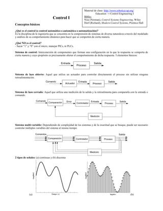
Sistema de control: Interconexión de componentes que forman una configuración en la que la respuesta se comporta de
cierta manera y cuyo propósito es precisamente alterar el comportamiento de dicha respuesta. 3 elementos básicos:
Sistema de lazo abierto: Aquel que utiliza un actuador para controlar directamente el proceso sin utilizar ninguna
retroalimentación.
Sistema de lazo cerrado: Aquel que utiliza una medición de la salida y la retroalimenta para compararla con la entrada o
comando.
Sistema multi-variable: Dependiendo de complejidad de los sistemas y de la exactitud que se busque, puede ser necesario
controlar múltiples variables del sistema al mismo tiempo.
2 tipos de señales: (a) continuas y (b) discretas
(a) (b)
Material de clase: http://www.robotica-up.org/
Education → Control Engineering I
Biblio:
Nise (Norman), Control Systems Engineering, Wiley
Dorf (Richard), Modern Control Systems, Prentice Hall
2.
3. Block Diagrams
Signals System
Summing junction Pickoff point
Cascaded subsystems Parallel subsystems
Feedback systems
Moving blocks forward & backwards
Moving pickoff points forward & backwards
4. Modeling dynamic systems
I. Electric systems
Component Voltage-current Current-voltage Voltage-charge Impedance Z(s) Admittance Y(s)
Operational amplifiers (Opams)
Inverting Opam Non-inverting Opam
)(
)(
)(
)(
1
2
sZ
sZ
sV
sV
i
o
−=
)(
)()(
)(
)(
1
21
sZ
sZsZ
sV
sV
i
o +
=
Summing inverting Opam Potentiometer
∑=
⎟⎟
⎠
⎞
⎜⎜
⎝
⎛
−=
N
i
i
i
f
f V
Z
Z
V
1 max21
22
1
2
)(
)(
θ
θ
=
+
==
RR
R
R
R
sV
sV
6. III. Rotacional mechanical systems
(a) (b) (c) (d)
(a): Solid cylinder around axis:
2
2
1
mrJ =
(b): Solid sphere:
2
5
2
mrJ =
(c):Rod about center:
2
12
1
mLJ =
(d):Rod about end:
2
3
1
mLJ =
Gear system Rack and pinion
(Radial to linear motion)
2
1
2
1
1
2
T
T
N
N
==
θ
θ
θrx =
Moment of inertia: Defined as the product of the mass k-times the
square of perpendicular distance to the rotation axis: I = kmr2
L
7. Derivation of a Schematic for a DC Motor
Current-carrying wire in a magnetic field
a. Current-carrying wire on a rotor; b. current-carrying wire on a rotor with commutation
and coils added to the permanent magnets to increase magnetic field strength
dt
d
ktV m
bb
θ
=)(
kb: emf constant
)()( tiktT aTm =
kT: motor torque constant
DC motor circuit diagram
8. Modeling of a Pneumatic cylinder
Mechanical part:
( )atmPPSMgkx
dt
dx
b
dt
xd
M −=+++2
2
where:
M : moving mass
x : rod’s position
b : viscous friction
k : spring constant
S : rod’s area
P : internal pressure
Patm: atmospheric pressure
g: gravity
Pneumatic part:
Modeling is based on the following classic hypotheses:
• The air is a perfect gas,
• The process is adiabatic,
• The actuator’s internal temperature is constant and homogeneous,
• The main chamber’s pressure is homogeneous due to its dimension,
• The servovalve’s response time is negligible.
dt
dx
V
PS
dt
dM
V
RT
dt
dP γγ
−=
where :
P: pressure
dt
dM
: mass input flow,
T : temperature R : air constant
γ : specific heat ratio V : chamber’s volume
9. State Space Representation
So, we have seen that dynamic systems are represented by a set of n differential equations:
mmnn
mmnn
ububxaxaxax
ububxaxaxax
212122221212
111112121111
......'
......'
++++++=
++++++=
.
.
.
mnmnnnnnnn ububxaxaxax ++++++= ......' 112211
It is common (and more compact) to represent them in a matrix form:
⎥
⎥
⎥
⎦
⎤
⎢
⎢
⎢
⎣
⎡
⎥
⎥
⎥
⎦
⎤
⎢
⎢
⎢
⎣
⎡
+
⎥
⎥
⎥
⎥
⎦
⎤
⎢
⎢
⎢
⎢
⎣
⎡
⎥
⎥
⎥
⎥
⎦
⎤
⎢
⎢
⎢
⎢
⎣
⎡
=
⎥
⎥
⎥
⎥
⎦
⎤
⎢
⎢
⎢
⎢
⎣
⎡
mnmn
m
nnmnn
n
n
n
u
u
bb
bb
x
x
x
aaa
aaa
aaa
x
x
x
...
...
...
...
...
...
......
...
...
'
...
'
'
1
1
111
2
1
21
22221
11211
2
1
x’ = A x + B u
BuAxx +=' is called space state equation. Vector x is called the state vector and contains
the variables of interest of the system.
Similarly, the output in state space form can be represented by: DuCxy +=
(Note: It is common to find systems with D=0, so Cxy = )
Graphically:
10. Time response
First order systems
Time constant: The time that
it takes for a step response to
rise to 63% of its final value.
Rise time: The time it takes
to rise from 10% to 90% of
the magnitude of the step
response.
a
Tr
2.2
=
Settling time: The time
required to settle or to reach
steady-state.
a
Ts
4
=
Second order systems: Introduction
11. Performance of Second-Order Systems
Fig.1. Transient response due to damping ξ
Natural frequency ωn: Frequency
of oscillation of the system without
damping.
Damping ζ: is any effect, either
deliberately engendered or inherent
to a system, that tends to reduce the
amplitude of oscillations of an
oscillatory system.
ζ=Exponential decay frequency/
Natural frequency
Fig.2. Step response of a control system
Rise time: The time it takes to rise from
10% to 90% of the magnitude of the step
response
n
rT
ω
ξ 6.016.2 +
=
Peak response: Magnitude of the
overshoot
2
1/
max 1 ξξπ −−
+= eC
Peak time: Time required to reach the
maximum overshoot
2
1 ξω
π
−
=
n
pT
Settling time: The time required to settle
or to reach steady-state.
n
sT
ξω
τ
4
4 ==
13. Practica 1- Introducción a Matlab
Temario:
- Introducción a Matlab (Editor Matlab, Simulink y Command Window)
- Transformada de Laplace
- Transformada Inversa de Laplace
- Derivar con Matlab
- Integrar con Matlab
- Vectores y Matrices
- Operaciones con matrices: suma, multiplicación, producto punto, inversa,
transpuesta, determinante,…
- Polinomios
- Operaciones con polinomios: suma, convolución, deconvolución, raíces,
reconstrucción de polinomio a partir de raíces, evaluación polinomial, …
- Señal continua
- Señal discreta
- Opciones de graficación: plot, subplot, colores, linewidth, strings,…
- Respuesta a un escalón e impulso
- Simulink: construcción de diagramas de bloques
************************************************************
Matlab:
1- Encuentre la transformada de Laplace de las siguientes expresiones:
a) tt
etety 22
25.15.325.1)( −−
++−=
b) )º604(5)º453cos(5)( 22
+++= −
tsentettty t
2- Grafique la evolución temporal y(t) de las siguientes expresiones:
a)
)23(
444
)( 22
2
++
++
=
sss
ss
sY
b)
)75)(38)(8(
564
)( 22
23
+++++
+++
=
sssss
sss
sY
3.- Resuelva las siguientes ecuaciones:
a) )72)(26)(15)(2( 23
++++= xxxxxy
b)
6.20
7.31148.4036.1306.19
2
234
−
−−++
=
x
xxxx
y
c) ¿Cuáles son las raíces de b ? Num/Den
14. d)
3388
1
)7756)(657681(
)536249)(14(56
)1( 2223
23
++
+
+++++
++++
=−=
xxxxxxx
xxxx
xY
c) Considere:
⎥
⎥
⎥
⎦
⎤
⎢
⎢
⎢
⎣
⎡
−−
=
012
891
321
A y
⎥
⎥
⎥
⎦
⎤
⎢
⎢
⎢
⎣
⎡
−=
567
101
654
B
c.1) 2A+B
c.2) A*B
c.3) AT
-B
c.4) det(A)/det(B)
4.- Para cada una de las funciones de transferencia siguientes obtener la respuesta
a un escalón unitario:
(a)
72
1
)( 2
++
=
ss
sH (b)
)8)(7(
10
)(
++
=
ss
sG (c)
1598
2
23
+++
+
sss
s
5.- Considere los siguientes sistemas:
15.0
1
)( 21
++
=
ss
sH
45.0
1
)( 22
++
=
ss
sH
Compare (eso quiere decir las 2 graficas en una misma figura) la respuesta a un escalón
del sistema en lazo abierto y lazo cerrado.
(Lazo cerrado: Hacerlo automático con feedback)
************************************************************
Simulink:
6.- Considere el diagrama de bloques de la siguiente figura.
(1) Obtenga en Simulink la respuesta de C(s) cuando R(s) es un escalón unitario
(2) Reduzca la función a un solo bloque y compruebe su resultado con el obtenido en (1)
15. Practica 2 – Modelado de Sistemas
1.- Considere un circuito RCL en serie con R=L=C=1.
a) Simule este sistema en Simulink y obtenga el comportamiento de la corriente y el
voltaje en el capacitor para un voltaje de alimentación de 1V.
b) ¿Cuál es el efecto de variar (i.e aumentar/disminuir) R en el voltaje y la corriente?
(Intente R=3Ω y R=0. 5Ω)
c) ¿Y de variar C? (Intente C=0.5, C=0.25, C=1.25, C=1.5)
d) Con los valores iniciales de R=L=C=1, ¿Cuál es la frecuencia de carga del capacitor?
2.- Modele un sistema masa-resorte-amortiguador con M=2 kg, fv=0.7, k=1. Explique
las respuestas de aceleración, velocidad y posición.
3.- Modele el siguiente sistema en Simulink y compare las velocidades y posiciones de
ambos vehículos con: M1=1kg, fv= 0.0196, k=1, M2=0.5 kg.
4.- Considere el sistema mecánico de traslación de la sig. figura. Simule este sistema en
Simulink y obtenga la evolución temporal de la posición y la velocidad para las tres
masas: x1(t), x2(t), x3(t) y v1(t), v2(t), v3(t).
5.- Modele el comportamiento de un motor de DC sin carga con L=1, R=4, k=0.031,
Jm=0.2, D=0.001.
6.- Compare el comportamiento de las 3 posiciones angulares del sig. sistema:
16. Practica 3
1. Encuentre H(s) a partir de la gráfica y compruebe sus resultados en Matlab/Simulink.
(a) (b)
(c) (d)
Sol: a)
3
18
+s
, b)
40
80
+s
, c)
92
9
2
++ ss
, d)
92
3
2
++ ss
2.- Use Matlab para construir el diagrama de polos y ceros de:
2746
22
)( 234
2
++++
++
=
ssss
ss
sH
3.- Encuentre el voltaje en el capacitor si el switch se cierra en t=0. Asuma condiciones iniciales iguales a cero.
De su gráfica en Matlab encuentre: a) la constante de tiempo, b) el tiempo de levantamiento, c) el tiempo de
asentamiento y d) el voltaje final del capacitor. Sol: a) 2 , b) 1.1s , c) 2s , d) 5V
4.- Determine la validez de una aproximación a 2º grado para:
a)
)20)(10)(5.6(
)7(71.185
)(
+++
+
=
sss
s
sH
b)
)20)(10)(9.6(
)7(14.197
)(
+++
+
=
sss
s
sH
Sol: (a) No es valido, e>5% , (b) Es valido, e=1.5%
17. Trabajos de Implementación
1.- Amplificadores Operacionales (Opams)
Fecha de entrega: La siguiente clase al 2° examen parcial.
Diseñe en Simulink e implemente en circuito:
a) Un derivador
b) Un integrador
c) Un circuito que haga la función: 321 5.02 uuu ++ donde u1, u2 y u3 son señales
independientes de entrada.
2.- Neumática
Fecha de entrega: Fin de curso
Considere 2 pistones neumáticos en configuración antagonista y un bloque de madera (o
cualquier otro material) entre ellos:
Diseñe un sistema de control de tal forma que, con la dinámica del sistema, el bloque
nunca se caiga:
Pistón-1 Pistón-2Bloque