Dynamic Vibration Absorber Design and Analysis
•
2 j'aime•2,697 vues

The document describes the mathematical modeling and analysis of a dynamic vibration absorber system. It presents the differential equations of motion for a primary system attached to a secondary absorber system. It then derives the frequency response equation and shows that tuning the natural frequencies of the two systems eliminates vibration response. MATLAB code is also included to simulate and analyze the time response and frequency response of the tuned dynamic vibration absorber.

Recommandé
Contenu connexe
Tendances
Tendances (20)
Similaire à Dynamic Vibration Absorber Design and Analysis
Similaire à Dynamic Vibration Absorber Design and Analysis (20)
Dernier
Dernier (20)
Dynamic Vibration Absorber Design and Analysis
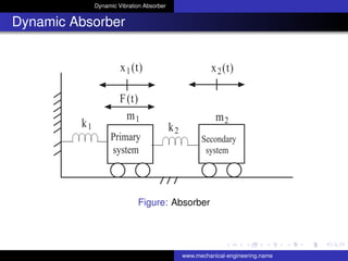
- 1. Dynamic Vibration Absorber Dynamic Absorber F(t) x1(t) m1 k1 k2 m2 x2(t) Primary system Secondary system Figure: Absorber www.mechanical-engineering.name
- 2. Dynamic Vibration Absorber Differential equations of motion From free body diagrams of the masses m1 and m2 m1¨x1 = −k1x1 − k2 (x1 − x2) + Feqsinωt m2¨x2 = k2 (x1 − x2) . (1) Rearranging the Eq.(1) m1¨x1 + (k1 + k2) x1 − k2x2 = Feqsinωt m2¨x2 + k2x2 − k2x1 = 0 . (2) www.mechanical-engineering.name
- 3. Dynamic Vibration Absorber Formulas For steady state solution, assume solution x1 = X1 sin ωt and x2 = X2 sin ωt. Substituting for x1 and x2 and their second time derivatives in Eq.(2), we obtain k1 + k2 − mω2 X1 − k2X2 sin ωt = Feqsinωt −k2X1 + k2 − m2ω2 X2 sin ωt = 0 . (3) Collecting out common terms and also because sin ωt = 0 at all time, we get k1 + k2 − mω2 X1 − k2X2 = Feq −k2X1 + k2 − m2ω2 X2 = 0 . (4) www.mechanical-engineering.name
- 4. Dynamic Vibration Absorber Cramer’s rule Solving for X1 and X2 using Cramer’s rule, we obtain X1 = Feq −k2 0 k2 − m2ω2 ∆ω , X2 = k1 + k2 − mω2 Feq −k2 0 ∆ω (5) The frequency equation is given by ∆ω = k1 + k2 − mω2 −k2 −k2 k2 − m2ω2 (6) which semplifies to ∆ω = 0 ⇒ m1m2ω4 − [(k1 + k2) m2 + k2m1] ω2 + k1k2 = 0 (7) www.mechanical-engineering.name
- 5. Dynamic Vibration Absorber Frequency equation Dividing out Eq. (7) by k1k2 m1m2 k1k2 ω4 − k1 + k2 k1 m2 k2 + m1 k1 ω2 + 1 = 0 . (8) In Eq.(8) the natural frequency of the main system is ω11 = k1/m1; auxiliary system is ω22 = k2/m2. The Eq.(8) may be rewritten as ω ω11 2 ω ω22 2 − 1 + k2 k1 ω ω22 2 + ω ω11 2 + 1 = 0 . (9) www.mechanical-engineering.name
- 6. Dynamic Vibration Absorber Dynamic Absorber When the main system and auxiliary system have same natural frequency ω11 = ω22, let ω ω11 = r ω ω22 = r . (10) Letting m2/m1 = µ, Eq.(10) reduces to r4 − (2 + µ) r2 + 1 = 0 . (11) www.mechanical-engineering.name
- 7. Dynamic Vibration Absorber Dynamic Absorber The new resonance frequencies of tuned system depend on the mass ratio µ. Let us assume that the resonance occurs at r ≡ r1 = ω ω11 r ≡ r2 = ω ω22 . (12) where the two roots are given by r2 1 , r2 2 = 2 + µ 2 ± 1 2 (2 + µ)2 − 4 . (13) or r2 1 , r2 2 = 1 + µ 2 ± 1 + µ 2 2 − 1 . (14) When ω11 = ω22, the natural frequencies are given by ω ω11 2 = 1 + µ 2 ± 1 + µ 2 2 − 1 . (15) www.mechanical-engineering.name
- 8. Dynamic Vibration Absorber Tuned condition Solving the determinants in Eq.(5) we have X1 = Feq k2 − m2ω2 ∆ω = Feq k2 − m2ω2 k1 + k2 − m1ω2 k2 − m2ω2 − k2 2 X2 = Feqk2 ∆ω = Feqk2 k1 + k2 − m1ω2 k2 − m2ω2 − k2 2 . (16) www.mechanical-engineering.name
- 9. Dynamic Vibration Absorber Tuned condition Under tuned condition, substituting k2 = m2ω2, the Eq.(16) gives X1 = Feq · 0 k1 + k2 − m1ω2 · 0 − k2 2 = 0 X2 = Feqk2 k1 + k2 − m1ω2 · 0 − k2 2 = − Feq k2 . (17) X2 = − Feq k2 ⇒ −X2k2 = Feq . (18) Fspring = Fexternal www.mechanical-engineering.name
- 10. Dynamic Vibration Absorber Application A machine runs at 5500 rpm. Its forcing frequency is very near to its natural frequency. If the nearest frequency of the machine is to be at least 20 per cent from the forced frequency, design a suitable vibration absorber for the sistem. Assume the mass of the machine as m1 = 30 kg. www.mechanical-engineering.name
- 11. Dynamic Vibration Absorber Application The natural frequency of the system at 478 rpm is ωn = 2π 478 60 ≈ 50 rad/s . (19) For 20 per cent variation, we obtain r1 = ω ωn = 0.8 r2 = ω ωn = 1.2 . (20) From Eq. (11) we have 0.84 − (2 + µ) 0.82 + 1 = 0 ⇒ µ = 0.202 . (21) Mass of auxiliary system is m2 = µ ⇒ m1 = 0.202 × 30 = 6.06 kg . (22) Stiffness values k1 =ω2 n × m1 = 502 × 30 = 75000 N/m ⇒ k2 = ω2 n × m2 = 502 × 6.06 = 15150 N/m . (23) www.mechanical-engineering.name
- 12. Dynamic Vibration Absorber Matlab: Main tspan = 0 : 0.05 : 10; y0 = [0; 0; 0; 0]; [t, y] = ode23( Dabsorber , tspan, y0); subplot(211); plot(t, y(:, 1)); xlabel( t(Solid line : x1(t)Dotted line : xd1(t)) ) holdon; plot(t, y(:, 2), −− ); subplot(212); plot(t, y(:, 3)); xlabel( t(Solid line : x2(t)Dotted line : xd2(t)) ); hold on; plot(t, y(:, 4), −− ); www.mechanical-engineering.name
- 13. Dynamic Vibration Absorber Matlab: Function function f = Dabsorber(t, y) m1 = 30; m2 = 0.202 ∗ m1; omegan = 50; k1 = omegan ∗ omegan ∗ m1; k2 = omegan ∗ omegan ∗ m2; omega = 15 ∗ 2 ∗ pi; Feq = 10; F = Feq ∗ sin(omega ∗ t); f = zeros(4, 1); f(1) = y(2); f(2) = F/m1 − ((k1 + k2)/m1) ∗ y(1) + (k2/m1) ∗ y(3); f(3) = y(4); f(4) = (k2/m2) ∗ y(1) − (k2/m2) ∗ y(3); www.mechanical-engineering.name
- 14. Dynamic Vibration Absorber Matlab: FRF clear all clc m1 = 30; m2 = 0.202 ∗ m1; omegan = 50; k1 = omegan ∗ omegan ∗ m1; k2 = omegan ∗ omegan ∗ m2; Feq = 10; k = 31; X1 = zeros(k, 1); X2 = zeros(k, 1); omega = zeros(k, 1); www.mechanical-engineering.name
- 15. Dynamic Vibration Absorber Matlab: FRF for m = 1 : k omega(m) = m; Deltaomega = m1 ∗ m2 ∗ omega(m)4 − ((k1 + k2) ∗ m2 + k2 ∗ m1) ∗ omega(m)2 + k1 ∗ k2; X1(m) = Feq ∗ (k2 − m2 ∗ omega(m)2)/Deltaomega; X2(m) = Feq ∗ k2/Deltaomega; end plot(omega, X1, omega, X2); legend( X1, X2); grid; xlabel( Frequency ); ylabel( Amplityde ); title( Frequency Response Functions ); www.mechanical-engineering.name
- 16. Dynamic Vibration Absorber Time history 0 2 4 6 8 10 −10 −5 0 5 10 t(Solidline: x1(t) Dottedline: xd1(t)) 0 2 4 6 8 10 −100 −50 0 50 100 t(Solidline: x2(t) Dottedline: xd2(t)) Figure: Time history www.mechanical-engineering.name
- 17. Dynamic Vibration Absorber Time history 0 2 4 6 8 10 −2 −1.5 −1 −0.5 0 0.5 1 1.5 2 primary system secondary system Figure: Time history www.mechanical-engineering.name
- 18. Dynamic Vibration Absorber FRF 0 50 100 150 200 −5 0 5 10 x 10 −3 Frequency [rad/s] Amplityde Frequency Response Functions X1 X2 Figure: Frequency Response Function www.mechanical-engineering.name