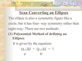
1. Scan Converting an Ellipses
The ellipse is also a symmetric figure like a
circle, but it has four- way symmetry rather than
eight-way. There are two methods:
(1) Polynomial Method of defining an
Ellipses
It is given by the equation:
(x - h)2 + (y - k)2 = 1
a2 b2

2. where (h, k) = ellipse center
a = length of major axis
b = length of minor axis
y
Center(h, k)
b a
k
h x

3. When the polynomial method is used to
define an ellipse, the value of x is
incremented
from h to a. For each step of x, each value of
y
is found by evaluating the expression.
y = b 1 – (x – h)2 + k
a2
This method is very inefficient, because the
square of a and (x – h) must be found; then
floating-point division of (x-h)2 by a2 etcs….

4. (2) Trigonometric method of defining an
Ellipses:
The following equations define an ellipse
trignometrically :
x = a cos(θ) + h and y = b sin(θ) + k
Where (x, y) = the current coordinates
a = length of major axis
b = length of minor axis
θ = current angle

5. The value of θ is varied from 0 to π/2 radians.
The remaining points are found by symmetry.
y (acos(θ)+h, bsin(θ)+k)
b a
k θ
x
h

6. Ellipse Axis Rotation
Since the ellipse shows four-way symmetry, it
can easily be rotated 90°. The new equation is
found by trading a & b, the values which
describe the major & minor axes. The
equation is:
(x - h)2 + (y - k)2 = 1
b2 a2
a = length of major axis
b = length of minor axis

7. In trigonometric method the equations are:
x = b cos(θ) + h and y = a sin(θ) + k
Where (x, y) = the current coordinates
a = length of major axis
b = length of minor axis
θ = current angle
Assume that the ellipse is rotate through an
angle of 90º. This rotation can be
accomplished by rotating the x & y axis
α degrees.

8. Midpoint Ellipse Algorithm
This is an incremental method for scan
converting an ellipse that is centered at origin
in standard position i.e with its major & minor
axes parallel to coordinate system axis.
It is very similar to midpoint circle algorithm.
However, b’coz of the four-way symmetry
property we need to consider the entire
elliptical curve in the first quadrant.

9. Let’s first rewrite the ellipse equation and
define function f that can be used to decide if
the midpoint between two candidate pixel is
inside or outside the ellipse:
< 0 (x,y) inside
f(x,y) = b2x2 + a2y2 – a2b2 = 0 (x,y) on
> 0 (x,y) outside

10. xi xi+1
T
yi
b Slope = -1
S Part 1
Q
Part 2
yj
yj-1 U V
xj
a

11. Now divide the elliptical curve from (0,b) to
(a,0) into two parts at point Q where the slope
of the curve is –1.
Slope of the curve is defined by f(x,y) = 0 is
dy/dx = - fx/fy, where fx & fy are partial
derivatives of f(x,y) with respect to x & y.
We have fx = 2b2x, fy = 2a2y &
dy/dx = - 2b2x/ 2a2y. Hence we can monitor
the slope value during the scan-conversion
process to detect Q.

12. Out starting point is (0,b).
Suppose that the coordinates of the last scan
converted pixel upon entering step i are
(xi, yi). We are to select either T(x i +1,yi) or
S(x i +1, yi – 1) to be the next pixel. The
midpoint of T & S is used to define the
following decision parameter.
pi = f (x i +1, yi – ½)

13. pi = b2(x i +1)2 + a2(yi – ½)2 – a2b2
If pi < 0, the midpoint is inside the curve, &
we choose pixel T.
If pi > 0, the midpoint is outside or on the
curve, & we choose pixel S.
Decision parameter for the next step is:
pi +1 = f (x i +1 + 1, yi +1 – ½)
= b2(x i +1 + 1)2 + a2(yi +1 – ½)2 – a2b2
Since x i +1 = xi + 1, we have

14. pi +1- pi = b2[(xi +1 + 1)2 - xi +12]
+ a2[(yi +1 – ½)2 – (yi – ½)2]
pi +1 = pi +2b2xi +1 + b2 + a2[(yi +1 – ½)2 –
(yi – ½)2]
 If T is chosen pixel (meaning pi < 0), we
have yi +1 = yi
If S is chosen pixel (meaning pi > 0), we
have yi +1 = yi – 1. Thus we can express
pi +1 in terms of pi and (xi +1, yi +1 ):

15. pi +1 = pi + 2b2xi+1 + b2 if pi < 0
pi + 2b2xi+1 + b2 – 2a2yi+1 if pi > 0
The initial value for this recursive expression
can be obtained by evaluating the original
definition of pi with (0,b):
p1 = b2 + a2(b – ½)2 – a2b2
= b2 – a2b + a2/4
We now move on to derive a similar formula
for part 2 of the curve

16. Suppose pixel (xj, yj) has just been scan
converted upon entering step j. The next pixel
is either U(xj, yj-1) or V(x j +1, yj – 1). The
midpoint of the horizontal line connecting U
& V is used to define the decision parameter.
qj = f (x j + ½, yj – 1)
qj = b2(x j + ½)2 + a2(yj – 1)2 – a2b2
If qj < 0, the midpoint is inside the curve, &
we choose pixel V.

17. If qj > 0, the midpoint is outside or on the
curve, & we choose pixel U. Decision
parameter for the next step is:
qj +1 = f (x j +1 + ½, yj +1 – 1)
= b2(x j +1 + ½)2 + a2(yj +1 – 1)2 – a2b2
Since yj +1 = yj - 1, we have
qj +1- qj = b2[(xj +1 + ½)2 – (xj +½)2] +
a2[(yj +1 – 1)2 – (yj+1)2]
qj +1 = qj + b2 [(xj +1 + ½)2 – (xj +½)2]
- 2a2yj+1 + a2

18.  If V is chosen pixel (meaning qj < 0), we
have xj +1 = xj + 1
If U is chosen pixel (meaning pi > 0), we
have xj +1 = xj. Thus we can express
qj +1 in terms of qj and (xj +1, yj +1 ):
qj +1 = qj + 2b2xj+1-2a2yj+1 + a2 if qj < 0
qj - 2a2yj+1 + a2 if qj > 0
The initial value for this recursive expression
is computed using the original definition of qj

19. And the coordinates (xk, yk) of the last pixel
chosen for part 1 of the curve:
q1 = f (xk + ½, yk – 1)
= b2(xk + ½)2 – a2(yk – 1)2 - a2b2
Algorithm:
int x=0, y=b; (starting point)
int fx =0, fy = 2a2b (Initial partial derivative)
int p = b2 – a2b + a2/4

20. while (fx < fy) /* |slope| < 1 */
{ setPixel(x,y)
x++;
fx = fx + 2b2;
if (p < 0)
p = p + fx + b2;
else {
y--;
fy = fy – 2a2;

21. p= p + fx + b2 – fy;
}
}
setPixel(x,y); /* set pixel at (x k,yk) */
p = b2(x+0.5)2 + a2(y-1)2 - a2 b2;
while (y > 0) {
y--;
fy = fy – 2a2;
if (p >= 0)

22. p = p – fy + a2;
else {
x++;
fx = fx + 2b2;
p = p + fx – fy +a2;
}
setPixel(x,y);
}