FINANCIAL MANAGEMENT

1. BREAK-
EVEN
ANALYSI

2. GROUP MEMBERS
• Ankita Srivastava
• Ayushi Srivastava
• Hrishikesh Pandey
• Ravi Kant
• Shivam Singh
• Sonali Mishra

3. Break even analysis
(B.E.A)
B.E.A. is an important tool of managerial
decision making. It is basically an analysis of
cost , revenue and profit with respect to
output produced and sold. But it is an
important practical tool to determine the
amount of profit for different levels of
output or sales.

4. BREAK EVEN POINT : It is the point of intersection
between total cost and total revenue lines , after
which profit start.
OR
It is the total minimum level of output or sales which
is necessary to avoid losses.

5. Assumptions
Fixed cost remains fixed and does not change for a reasonable
degree of output change.
 variable cost changes at a constant rate . In other worlds,
average variable cost is constant and is equal to the marginal
cost. (AVC= MC)
BEP is based on the assumption of constant input costs. It
means that if the firm decides to produce more or less , the
average variable cost of input remains constant.
The BEP analysis assumes that prices of a product or products
to be manufactured by a firm do not change by a change in
output. It means that whatever the firm produces, it can be
sold at the same price and it is not required to reduce price if
it wants to sell more.

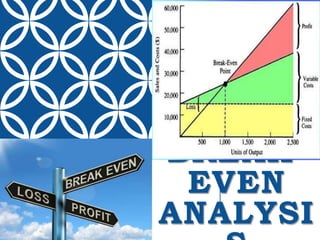
6. In figure fixed cost is constant and indicated by a horizontal line PQ . While
total cost is combination of fixed cost and variable cost . The total cost
curve is an upwardly reclining straight line indicating that it is increasing at
a constant rate (marginal cost is constant). Total revenue curve is an upward
going straight line starting from the point of origin O. it implies that the
total revenue is increasing at a constant rate(due to constant price). Initially
the T.C.>T.R. so firm suffers losses. When output reaches M level of output
losses vanish and if output Is greater than M profits are earned. M level of
output is called break even point or break even output level.

7. Methods of break even
analysis
There are three ways of doing break even analysis.
These methods are :
 Mathematical method
 Graphical method
 Accounting method

8. 1. Mathematical Method
Since break even analysis is based on constant AVC and constant
price a mathematical equation can be very conveniently used to
find out the level of output where total cost is equal to total
revenue or where profit or loss is zero.
Mathematical Review : A firm is engaged in a business where
the price of the product is Rs. 10 per unit , the average
variable cost is Rs 8 and fixed cost is Rs. 5000 per month.
The firm want to know the minimum level of output which it
must sell to avoid losses.
Solution : we assume that break even output is ‘X’.
Total revenue(T.R.) = 10*X
Total variable cost(T.V.C.) = 8*X
Fixed cost(F.C.) = 5000
Total cost(T.C.) = 5000+8*X

9. We know that at break even level
Total revenue = Total cost
10*X = 5000+8*X
10*X-8*X = 5000
2*X = 5000
X = 5000/2
X = 2500 Units
Therefore , the firm must sell at least 2500 units per month to avoid
losses , because at 2500 units
Total revenue=10*2500
Total revenue = Rs. 25000
Total cost = 5000+2500*8
Total cost = 5000+20000
Total cost = Rs.25000
If actual output is greater than 2500 units then firm will make profit
and if output is less than 2500 units it will be in loss.
Suppose actual output is 3000 units then,
T.R. = 3000*10
T.R. = Rs 30000

10. T.C. = 5000+3000*8
T.C. = 5000+24000
T.C. = Rs 29000
PROFIT = T.R. –T.C.
PROFIT = 30000-29000
PROFIT = Rs 1000
Hence at this level of output firm makes profit of Rs. 1000 which keep
increasing as out put increases.
Impact of change of price, cost and fixed costs
1. Suppose price increases by Rs 2 then,
T.R. = 12*X
T.C. = 5000+8*X
T.R, = T.C.
12*X = 5000+8*X
4*X = 5000
X = 1250 UNITS
Thus increase in price of product lower the break even point (possible
only when price is greater than AVC) .

11. 2. When average variable cost decreases
Suppose AVC is Rs. 7.50
T.R. = 10*X
T.C. = 5000+7.50*X
10*X = 5000+ 7.50*X
2.50*X = 5000
X = 2000 Units
When AVC decreases the BEP also decrease.(it is possible only as long as
the AVC is lower than the price)
3. Impact of fixed cost
Suppose fixed cost increases to Rs 8000.
T.R. = 10*X
T.C. = 8000+8*X
T.R. = T.C.
10*X = 8000+8*X
2*X = 8000
X = 4000 Units
Now firms new break even output is 4000 units which increase as
the F.C. increases.

12. 2. Graphical Method
The graphical method can also be used to determine all
the variables that we find by the mathematical method.
The graphical method is used to give visual impact
rather than accurately measure the BEP, or the profit
or cost . We know that the use of graphs facilitates our
understanding of a phenomenon and presents a
complete picture in one view , so that the pattern of
different variables and their inter-relationship can be
easily understood.

13. In this figure the slop of T.R. and T.C. curves indicates price and AVC
respectively. Hence if there is an increase in price the slop of the T.R.
line will increase and vice-versa. Similarly , the change in AVC will be
presented by the change in the slop of the T.C. line. An increase in slope
means a rise in AVC and vice versa . The change in fixed cost will be
indicated by the upward or downward shift of the F.C. line.
M is break even point where T.C. and T.R. line intersect each other.
Fixed cost

14. In this way by making changes in an appropriate manner , any new
break-even point can be shown by the graphical method.
The total amount of profit is shown by the vertical distance between the
T.R. and T.C. curves. A profit curve/line can be shown graphically
which will show the level of profit at different levels of output.
Break even graph can be shown in purely monetary term also. In the
above figure , we are measuring output on X axis by physical units .

15. However output on ‘X’ axis can be shown by monetary units also that is
sales. If we take sales in rupees on ‘X’ axis and use the same scales as
on ‘Y’ axis , then T.R. curve will be 450 line passing through the point
of origin as shown below :

16. In such situation sales shown on ‘X’ axis are always equal to
revenue on the ‘Y’ axis . Here the B.E.P. point shows that
at the given level of sales , cost is equal to this value . If
the sales are greater than this value , there is profit and if
sales are less than this value , there is losses.
It can be concluded that this method is not very suitable for
making accurate measurements. However , it is
commonly used for its visual impact . That is showing a
total picture of different relationships in one glance.

17. 3. Accounting method
Accounting method is based on readily available accounting
information that is total value of sales , total variable cost and the
fixed cost . This is also called as “contribution method” . It is
nothing but the difference between sales value and variable cost.
It is gap which is used to meet the fixed cost . Break-even is meet
as soon as this gap is equal to fixed cost. At a low output level,
the total value of this gap is low and hence it is less than fixed
cost, but as soon as sales increases the absolute value of this gap
becomes high and it is equal to the fixed cost and the break-even
point is reached. If sales continue further , the gap is greater
than the fixed cost , which result in net profit to the firm.
From this view point, BEP find when
Total contribution = Fixed cost
Another way of looking up is called contribution per unit of output
that is,
BEP = F.C./Contribution per unit

18. Contribution per unit is the unit difference between price and
average variable cost.
As soon as this contribution accumulates to the total fixed cost , the
break-even is reached. If output continues further, this
contribution will result in net profit to the firm.
This can be understand by an example-
Firm cost details :
• Material cost per unit Rs. 2
• Labor cost per unit Rs. 3
• Power expenses per unit Rs. 1
• Rent o building Rs 4000 P.M.
• Depreciation and intt. Rs. 2000 P.M
• Management exp. Rs. 5000 P.M.
Product is expected to be sold for Rs 8 per unit.
Solution :
We know that first three items are variable cost while last three are
fixed cost.

19. So, AVC = 2 + 3 + 1
AVC = 6
F.C. = 5000 + 4000 + 2000
F.C. = 11000
Price = Rs. 8
Contribution per unit = Price - AVC
= 8 - 6
= Rs 2
Break even point = 11000/2
= 5500 Units
Break even sales = 5500*8
= Rs 44,000
Break even cost = 11000 + 5500*6
= Rs 44,000
The firm required to make turnover of Rs 44,000 per month, to be
able to avoid losses. At this level total variable cost is Rs 33000
and total contribution of Rs 11,000 is just equal to the fixed cost.

20. P.V RATIO or Profit volume ratio
This concept of P/V ratio is very useful tool in BEP analysis. This is
more commonly used because many times, the variable cost and
the sales figures are available only in aggregate and not on a per
unit basis. This is especially true for a multi-product firm .
P.V Ratio can be found by any of method—
P.V ratio = (price-AVC)/price
= (sales- variable cost)/sales
= (fixed cost+profit)/sales
= change of profit/change of sale
B.E.P=F.C./P.V ratio
Example-1 : A multiproduct firm estimates that when it starts its
operations, the fixed cost is expected to be Rs 80,000 per month,
while variable cost is expected to be Rs 40,000 . The firm expects
to sell this output for Rs 50,000 . What is minimum level of sales
that the firm should avoid losses.

21. Solution : P.V Ratio = (sales-variable cost)/sales
= (50,000 - 40,000)/50,000
= 10,000/50,000
= 0.2
Now, B.E.P = 80,000/0.2
= Rs 4,00,000
The firm must make a sale of 4,00,000 per month to avoid losses.
Example-2 : 2012 2013
sales (Rs) 8,00,000 10,00,000
T.C. (Rs) 7,50,000 9,00,000
Find p.v. ratio , fixed cost and profit if sales next year are expected to
be Rs 13,00,000.
Solution :
profit for 2012 = 8,00,000-7,50,000
= 50,000
profit for 2013 = 10,00,000-9,00,000
= 1,00,000
change in profit = 50,000

22. Change in sales = 2,00,000
1. P.V Ratio = change in profit/change in sales
= 50,000/2,00,000
= .25
2. P.V ratio = (F.C.+PROFIT)/SALES
.25 = (F.C.+50,000)/8,00,000
2,00,000 = F.C.+50,000
F.C. = 1,50,000
3. P.V ratio = (F.C. + PROFIT)/SALES
.25 = (1,50,000 + P)/13,00,000
P = 3,25,000-1,50,000
P = 1,75,000
In this examples , we have assumed constant price , AVC, and the
fixed cost.

23. Margin of safety
Margin of safety indicates that how far away is the firm
from the break-even point. In other words , what is the
excess of present sales over the break-even sales. The
higher the margin of safety of a firm , the greater is the
safety of firm from sales fluctuations .
Margin of safety = Present sales - BEP sales
Margin of safety ratio = Present sales - BEP sales
The margin of safety ratio indicates that how much decline
in sales can still keep the firm away from losses. Since it
is safe to work on the brink that is very close to break-
even point sales , it is always good to keep a safety
margin.

24. Uses and Applications of Break-Even
Analysis
 It provides us an easy tool to keep away from losses ,
which is the first consideration of any firm.
 It gives us a bird’s eye view of our revenue and cost
structure as well as the profit position.
 It is a useful tool to decide about the production
process.
 It can help us in choosing a better product mix.

25. Limitation of Break-Even Analysis
Break-even analysis is not free of its limitations . The limitations
come from its assumptions. It is said that :
 It is often not possible to divide costs into two categories that are
fixed and variable cost.
 The assumption of constant price and AVC may also not hold
good , if variable returns apply.
 Many firms are multi product firms, where it is not be possible
to precisely segregate the variable costs, especially when the
design , shape and size of products keep changing .
In spite of these limitations , it can be seen that the BEP is a very
useful tool of analysis for managerial decision making.