Yaroslav Rozhankivskyy: Три складові і три передумови максимальної продуктивн...
8071 25045-1-pb
1. www.ccsenet.org/ijbm International Journal of Business and Management Vol. 5, No. 11; November 2010
Oil Price Volatility, Global Financial Crisis and
The Month-of-the-Year Effect
Olowe, Rufus Ayodeji
Department of Finance, University of Lagos, Lagos, Nigeria
Tel: 234-80-2229-3985 E-mail: raolowe@yahoo.co.uk
Abstract
This paper investigates the month-of-the-year effect in the UK Brent crude oil market using the GARCH (1,5)
and GJR-GARCH (1,5) models in the light of Asian financial crisis and the global financial crisis using daily
data over the period, January 4, 1988 and May 27, 2009. The result shows the presence of the month-of-the-year
effect in volatility but not in the return in the oil market. However, the pattern of significance of monthly effect
in volatility is affected by the choice of model. The significant month-of-the-year effect on volatility may be in
line with information availability theory
The result shows that the Asian financial crisis has an impact on the oil price return series while the global
financial crisis has no impact on oil price returns. The Asian financial crisis and global financial crisis did not
account for the sudden change in variance.
Keywords: Month-of-the-year effect, Volatility, Oil prices, Global Financial crisis, Volatility persistence,
GARCH
JEL: F10, G14
1. Introduction
The monthly seasonality in returns has been well documented and tested for various stock markets and countries
(Rozeff and Kinney, 1976; Gultekin and Gultekin, 1983; Keim, 1983; Reinganum, 1983). The month-of-the-year
effect is present when returns in some months are higher than other months. This seasonal market anomaly, if
present, refutes market efficiency. Studies on monthly seasonality, also called January effect or year end effect or
“tax loss selling” hypothesis, argued that investors, in order to reduce their taxes, sell their stocks in December
(which is the tax month) to book losses. The selling of stocks by various investors will put downward pressure
on the prices. As soon as December ends market corrects and stock prices rise. The stocks will give higher return
in January. Wachtel (1942) was the first to point out the seasonal effect in the US markets. Rozeff and Kinney
(1976), Gultekin and Gultekin (1983), Keim (1983), Reinganum (1983) among others also provided evidence
supporting January effect in the USA. Berges, McConnell, and Schlarbaum (1984) and Tinic, Barone-Adesi and
West (1990) found seasonal effect in Canada. January effect has also been investigated for emerging markets
(Nassir and Mohammad, 1987; Ho, 1999; Fountas and Segerdakis, 1999; Kumar and Singh, 2008). Apart from
the stock market, seasonal effect has also been investigated for other commodity markets (Kumar and Singh,
2008) and the foreign exchange market with more focus on the day-of-the-week effect (McFarland et al., 1982;
Hilliard and Tucker, 1992; Cornett et al., 1995; Aydogan and Booth, 2003; and Yamori and Mourdoukow, 2003).
Little or no work has been done on monthly seasonality of the oil market.
Most studies on the seasonal effects concentrated more attention on seasonal pattern in mean return (see also
Jaffe and Westerfield, 1985; Solnik and Bousquet, 1990; Baronet, 1990, among others). An investor should be
concerned not only with variations in asset returns, but also the variances in returns. Engle (1993) argues that
risk-averse investors should reduce their investments in assets with higher return volatilities. Engle (1982)
introduced the autoregressive conditional heteroskedasticity (ARCH) to model volatility by relating the
conditional variance of the disturbance term to the linear combination of the squared disturbances in the recent
past. Bollerslev (1986) generalized the ARCH model by modeling the conditional variance to depend on its
lagged values as well as squared lagged values of disturbance, which is called generalized autoregressive
conditional heteroskedasticity (GARCH). Since the work of Engle (1982) and Bollerslev (1986), variants of the
GARCH models have been developed. Some of the models include IGARCH originally proposed by Engle and
Bollerslev (1986), GARCH-in-Mean (GARCH-M) model introduced by Engle, Lilien and Robins (1987),the
standard deviation GARCH model introduced by Taylor (1986) and Schwert (1989), the EGARCH or
Exponential GARCH model proposed by Nelson (1991), TARCH or Threshold ARCH and Threshold GARCH
156 ISSN 1833-3850 E-ISSN 1833-8119
2. www.ccsenet.org/ijbm International Journal of Business and Management Vol. 5, No. 11; November 2010
were introduced independently by Zakoïan (1994) and Glosten, Jaganathan, and Runkle (1993), the Power
ARCH model generalised by Ding, Zhuanxin, C. W. J. Granger, and R. F. Engle (1993) among others.
If investors can identify a certain pattern in volatility, then it would be easier to make investment decisions based
on both return and risk (Kiymaz and Berument, 2003). The understanding of seasonality in risk and returns is
important to financial managers, financial analysts and investors especially in assisting them in developing an
appropriate strategy in the context of the financial market. Thus, an investigation of the monthly seasonal effect
in returns should also consider the monthly seasonal effect on volatility. Several studies have been done using
the GARCH framework to investigate the seasonal effect. Berument and Kiymaz (2001) model seasonal effect
using GARCH model. Their findings show that the seasonal effect is present in both volatility and return
equations. Several studies have been done using the GARCH framework to investigate the seasonal effects
(Berument and Kiymaz, 2001; Choudhry, 2000; Balaban, Bayar and Kan, 2001; Kiymaz and Berument, 2003;
Yalcin and Yucel, 2006, Chandra, 2004; Apolinario, Santana, Sales and Caro, 2006 among others).Little or no
work has been done on the month-of-the-year effect in the crude oil market using GARCH models. This paper
attempts to fill this gap. The month-of-the-year effect in return contradicts the weak form of market efficiency,
which states that asset prices are random and it is not possible to predict asset price and return movements using
past price information. The understanding of the month-of-the-year effect in risk and returns is important to
financial managers, financial analysts and investors to develop appropriate strategy in the context of any
commodity or asset market.
The Asian Financial crisis of 1997 and the Global Financial crisis of 2008 could have affected oil price volatility.
The Asian Financial Crisis which began in 1997 was a period of financial crisis that affected much of Asia
raising fears of a worldwide economic meltdown due to financial contagion. The crisis started in Thailand on
July 2, 1997 with the devaluation of Thai baht caused by the decision of the Thai government to float the baht,
cutting its peg to the United States dollar, after being unsuccessful in an attempt to support it in the face of a
severe financial overextension that was in part real estate driven. Prior to the crisis, Thailand economy was in the
glimpse of collapse as it had acquired a burden of foreign debt. The crisis spread to other Southeast Asia
countries (Philippine, Malaysian, Indonesian, Singapore, South Korea, Hong Kong and Taiwan) and Japan with
their currencies slumping, stock markets collapsing and other asset prices declining, and a precipitous rise in
private debt. The Asian crisis made international investors reluctant to lend to developing countries, leading to
economic slowdowns in developing countries in many parts of the world. The economic slowdowns affected the
demand for oil reducing the price of oil, to as low as $8 per barrel towards the end of 1998, causing a financial
pinch in OPEC nations and other oil exporters. This reduction in oil revenue led to the 1998 Russian financial
crisis, which in turn caused Long-Term Capital Management in the United States to collapse after losing $4.6
billion in 4 months (Lowenstein, 2000).
The global financial crisis of 2008, an ongoing major financial crisis, could have affected stock volatility. The
crisis which was triggered by the subprime mortgage crisis in the United States became prominently visible in
September 2008 with the failure, merger, or conservatorship of several large United States-based financial firms
exposed to packaged subprime loans and credit default swaps issued to insure these loans and their issuers. On
September 7, 2008, the United States government took over two United States Government sponsored
enterprises Fannie Mae (Federal National Mortgage Association) and Freddie Mac (Federal Home Loan
Mortgage Corporation) into conservatorship run by the United States Federal Housing Finance Agency
(Wallison and Calomiris, 2008; Labaton and Andrews, 2008). The two enterprises as at then owned or
guaranteed about half of the U.S.'s $12 trillion mortgage market. This causes panic because almost every home
mortgage lender and Wall Street bank relied on them to facilitate the mortgage market and investors worldwide
owned $5.2 trillion of debt securities backed by them. Later in that month Lehman Brothers and several other
financial institutions failed in the United States (Labaton, 2008). The crisis rapidly evolved into a global credit
crisis, deflation and sharp reductions in shipping and commerce, resulting in a number of bank failures in
Europe and sharp reductions in the value of equities (stock) and commodities worldwide. In the United States,
15 banks failed in 2008, while several others were rescued through government intervention or acquisitions by
other banks (Letzing, 2008). The financial crisis created risks to the broader economy which made central banks
around the world to cut interest rates and various governments implement economic stimulus packages to
stimulate economic growth and inspire confidence in the financial markets. The financial crisis could have
affected the uncertainty in the demand for oil, thus, causing uncertainty in the price of oil.
The purpose of this paper is to investigate the month-of-the-year effect in the Crude Oil market using GARCH (1,
5) and GJR-GARCH (1, 5) models in the light of Asian and the global financial crises. The rest of this paper is
organised as follows: Section two discusses an overview of the Global oil market while chapter three discusses
Published by Canadian Center of Science and Education 157
3. www.ccsenet.org/ijbm International Journal of Business and Management Vol. 5, No. 11; November 2010
the literature review. Section four discusses methodology while the results are presented in Section five.
Concluding remarks are presented in Section six.
2. Overview of the Global Oil Market
Prior to the establishment of OPEC, the United States and British oil companies provided the world with
increasing quantities of cheap oil. The world price was about $1 per barrel, and during this time the United States
was largely self-sufficient, with its imports limited by a quota. In 1960, as a way of curtailing unilateral cuts in
oil prices by the big oil companies in the U.S and Britain, the governments of the major oil-exporting countries
formed the Organization of Petroleum Exporting Countries, or OPEC. OPEC’s goal was to try to establish
stability in the petroleum market by preventing further cuts in the price that the member countries - Iran, Iraq,
Kuwait, Saudi Arabia, and Venezuela - received for oil. The OPEC countries succeeded in stabilizing the oil
prices between $2.50 and $3 per barrel up till the early 70s. Apart from the four founding members of OPEC,
other countries later joined OPEC. The membership of OPEC has fluctuated overtime. Indonesia withdrew from
OPEC in January 2009, Angola joined OPEC in January 2007, Ecuador withdrew from OPEC in January 1993
and rejoined in November 2007, and Gabon withdrew from OPEC in July 1996. The current membership of
OPEC include Algeria, Ecuador, Iran, Iraq, Kuwait, Libya, Nigeria, Qatar, Saudi Arabia, United Arab Emirates,
and Venezuela. OPEC member countries agreed on a quota system to help coordinate its production policies,
but attempts to stabilize prices within a price band relied on producers having to constrain supply to create a tight
market, thus generating an economic disincentive to build stocks (UNCTAD, 2005). OPEC members benefit
from higher short-term prices; however, a tight market generates volatility and reduces the market’s ability to
respond to contingencies (UNCTAD, 2005). Furthermore, disagreements on production quotas and members'
mistrust have added to uncertainty and fuelled volatility.
The displacement of coal as a primary source of energy and development of internal-combustion engine and the
automobile led to increasing oil consumption throughout the world, especially in Europe and Japan, thus,
causing an enormous expansion in the demand for oil products.
The era of cheap oil came to an end in 1973 when, as a result of the Arab-Israeli War, the Arab oil-producing
countries cut back oil production and embargoed oil shipments to the United States and the Netherlands. This
raised prices fourfold to $12 per barrel. The Arab nations' cut in production, totaling 5 million barrels, could not
be matched by an increase in production from by countries (UNCTAD, 2005). This shortfall in production, which
represented 7 per cent of world production outside the USSR and China, caused shock waves in the market
especially to oil companies, consumers, oil traders, and some governments (UNCTAD, 2005). Furthermore, the
Iranian revolution in 1979 which led to a reduction in Iran's output by 2.5 million barrels of oil per day forced up
oil prices in 1979. The outbreak of war between Iran and Iraq in 1980 aggravated the situation in the world oil
market. The war led to a loss in oil production of 2.7 million barrels per day on the Iraqi side and 600,000 barrels
per day on the Iranian side. This force oil prices to increase to $35 per barrel (UNCTAD, 2005).
The high oil prices contributed to a worldwide recession which gave energy conservation a push reducing oil
demand and increasing supplies. There were significant increases in oil supplies from non-OPEC countries, such
as those in the North Sea, Mexico, Brazil, Egypt, China, and India. This forced down the oil prices. Attempts by
OPEC to stabilize prices during this period (after the Iran-Iraq war) were unsuccessful. The failure of OPEC to
stabilize prices during this period has been attributed to members of OPEC producing beyond allotted quotas
(UNCTAD, 2005). By 1986, Saudi Arabia had increased production from 2 million barrels per day to 5 million
barrels per day. This made oil prices to crash below $10 per barrel in real terms (UNCTAD, 2005). Oil prices
remain volatile despite various efforts by OPEC to stabilize prices. As at 1989, the Soviet Union increased its
production to 11.42 million barrels per day, accounting for 19.2 percent of world production in that year. This
led to further reduction in oil prices.
The invasion of Kuwait by Iraq leading to the Gulf War in 1990 caused prices to rise, but with the increasing
world oil supply, oil prices fell again, maintaining a steady decline until 1994. The lower oil prices brightened the
economies of United States and Asia, thus, boosting oil demand and prices rise again. The financial crisis in Asia
in 1997 caused economies in the region to grind to a halt. Oil demand fell and the surplus oil production pushed
down oil prices. Oil prices decreased to around $10 per barrel in late 1998. In 1999, there was a sudden increase
in demand which along with production cutbacks by OPEC raises oil prices to about $30 per barrel in 2000 but
they fell once again in 2001. However, since March 2002, oil prices have been on an upward trend climbing to
record level reflecting especially the developments related with the war in Iraq and increasing speculative trading
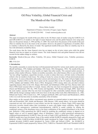
in oil futures on Futures exchanges. As at July 11, 2008, the crude oil prices per barrel of the UK Brent in
US$ per barrel was $143.68. Figure 1 shows the trend in daily oil prices since 1988. From July 14, 2008, oil
prices have been gradually falling possibly reflecting world economic recession. As at January 2, 2009, the crude
158 ISSN 1833-3850 E-ISSN 1833-8119
4. www.ccsenet.org/ijbm International Journal of Business and Management Vol. 5, No. 11; November 2010
oil prices per barrel of the UK Brent was $42.68. However since January 9, 2009, oil prices have been
fluctuating, rising to $61.28 per barrel as at May 27, 2009.
3. Literature Review
The market anomalies, which are proofs of market inefficiencies, have well documented in the finance literature.
Market anomalies show the existence of predictable behavior in stock returns may lead to profitable trading
strategies, and in turn, abnormal returns. The market anomalies that have attracted the attention of researchers
are broadly known as calendar or seasonal effects. The most popular seasonal effects studied are the day of the
week effect and the month-of-the-year or January effect.
The month-of-the-year effect is present when returns in some months are higher than other months. . In the USA
and some other countries, December is the year-end month and also the tax month. It is argued that investors will
sell shares that have lost values in December in order to reduce their taxes. The sale by various investors will put
a downward pressure on the share prices and thus lowers stock returns. As soon as the tax month (December)
ends, investors start buying shares in January and share prices will start rising. This will make stock returns to be
high in the month of January. This tax-loss selling hypothesis has been found to be consistent with the ‘year-end’
effect and the ‘January effect’ in stock returns by various studies (Kumar and Singh, 2008; Bepari and Mollik,
2009). Wachtel (1942) was the first to point out the seasonal effect in the US stock markets. Some other studies
in the USA supporting this effect include Rozeff and Kinney (1976), Keim (1983) and Reinganum (1983).
Rozeff and Kinney (1976) found that stock returns in January to be larger than in other months. Keim (1983)
found that small firm returns were significantly higher than large firm returns during the month of January.
Reinganum (1983), however, found that the tax-loss-selling hypothesis could not explain the entire seasonality
effect.
Seasonal effect has been found in other developed countries apart from United States. Gultekin and Gultekin
(1983) examined data of 17 industrial countries with different tax laws and confirmed the January effect. Berges,
McConnell, and Schlarbaum (1984) and Tinic, Barone-Adesi and West (1990) found seasonal effect in Canada.
Boudreaux (1995) found the presence of the month-end effect in markets in Denmark, Germany and Norway.
The seasonal effect in stock returns has also been found in UK (Lewis, 1989), Australia (Officer, 1975; Brown,
Keim, Kleidon and Marsh, 1983) and Japan (Aggarwal, Rao and Hiraki, 1990). Raj and Thurston (1994)
investigated the January and April effects in the New Zealand stock market and found no significant effect.
Nassir and Mohammad (1987) investigated the January effect in Malaysia and found the average January returns
to be significantly positive and higher than in other months. Ho (1999) found that six out of eight emerging
Asian Pacific stock Markets exhibit significantly higher daily returns in January than in other months. Other
studies include Fountas and Segerdakis (1999), Pandey (2002), Lazar et al. (2005), and Bepari and Mollik
(2009).
Apart from the stock market, the seasonal effect has also been investigated for other financial markets such as
the foreign exchange market. McFarland et al. (1982), Hilliard and Tucker (1992), Cornett et al. (1995),
Aydogan and Booth (2003) and Yamori and Kurihara (2004) investigated the day-of-the-week effect for the foreign
exchange market. Yamori and Kurihara (2004) investigated the day-of-the-week effect for 29 foreign exchange
markets in the 1980s and found the presence of the day-of-the-week effect. They also stated that the
day-of-the-week effect disappeared for almost all 29 countries in the 1990s. Little or no work has been done on
the day-of-the-week effect of the oil market.
Most of the studies on the seasonal effect discussed so far have focused attention on seasonal pattern in mean
return. An investor should be concerned not only with variations in asset returns, but also the variances in returns.
Engle (1993) argues that risk-averse investors should reduce their investments in assets with higher return
volatilities. Engle (1982) introduced the autoregressive conditional heteroskedasticity (ARCH) model which was
later generalized (GARCH) by Bollerslev (1986). The GARCH (p, q) model has p ARCH terms and q GARCH
terms and is given as :
p q
V2
t Z ¦D H
i 1
2
i t i ¦E V
j 1
2
j t j (1)
where, ı2 is conditional variance of İt and Ȧ 0, Į • 0 , ȕ • 0 . Equation (1) shows that the conditional variance is
explained by past shocks or volatility (ARCH term) and past variances (the GARCH term). Equation (2) will be
Published by Canadian Center of Science and Education 159
6. www.ccsenet.org/ijbm International Journal of Business and Management Vol. 5, No. 11; November 2010
4.2 Properties of the Data
Table 1 reports the preliminary statistics (evidence) for the oil price return series for the entire study period as
well as the return for each month of the year. The average return for the entire study period is 0.0002. The
standard deviation of the return is 0.0242, and skewness is -0.6872. The kurtosis is 17.763 which is much larger
than 3, the kurtosis for a normal distribution. The Jarque-Berra normality test rejects the normality of returns at
the 5 percent level. The negative skewness is an indication of a non-symmetric series. Figure 2 clearly show that
the distribution of the stock return series show a strong departure from normality.
When the return of each month is analyzed in Table 1, the findings indicate that December has a mean return of
0.08 percent, while January has a mean return of -0.15 percent. The signs of the returns are inconsistent with the
results of Rozeff and Kinney (1976), Keim (1983), Reinganum (1983) among others. The lowest return of -0.26
percent is observed for October while the highest return of 0.15 percent is observed for March. The lowest
standard deviation of 0.0192 is observed for July while the highest standard deviation of 0.0346 is observed for
January. March, April, June, July, August and November have positive skewness while all other months have
negative skewness. However, the impact of the negative skewness appears to be predominant as the overall
skewness is negative
The kurtosis for each month is larger than 3, the kurtosis for a normal distribution. The Jarque-Bera normality
test rejects the hypothesis of normality for the each month of the year.
The Ljung-Box test Q statistics as reported in Table 2 are all significant at the 5% for all reported lags
confirming the presence of autocorrelation in the stock return series. The Ljung-Box test Q2 statistics for are all
significant at the 5% for all reported lags confirming the presence of heteroscedasticity in the oil price return
series.
Table 3 shows the results of unit root test for the oil price return series. The Augmented Dickey-Fuller test and
Phillips-Perron test statistics for the oil price return series are less than their critical values at the 1%, 5% and
10% level. This shows that the oil price return series has no unit root. Thus, there is no need to difference the
data.
In summary, the analysis of the oil price return indicates that the empirical distribution of returns in the oil
market is non-normal, with very thick tails. The leptokurtosis reflects the fact that the market is characterised by
very frequent medium or large changes. These changes occur with greater frequency than what is predicted by
the normal distribution. The empirical distribution confirms the presence of a non-constant variance or volatility
clustering.
4.3 Models used in this Study
This study will attempt to model the volatility of daily oil price return using the GARCH (1, 5) and
GJR-GARCH (1, 5) models in the light of Asian financial crisis and the global financial crisis. Different models
including EGARCH model were initially tested in the study. The GARCH (1, 5) and GJR-GARCH (1, 5) models
were chosen on the basis of maximum log-likelihood or minimum Akaike information Criterion. The GARCH
(1,5) model will first be applied in investigating the volatility and month-of-the-year effect of the oil price
return series. Then, the GARCH (1,5) model and the and GJR-GARCH (1, 5) model will be augmented to
account for sudden change in variance in the volatility equation.
Thus, the mean and variance equations of the GARCH (1,5) model are given as :
11
Rt = b0+eRt-1+ ¦ b jG jt +g1ASF+g2GFC +İt H t / It 1 ~ N(0, V2 , v t )
t
(3)
j 1
5
V2
t h 0 D H 2 1
t ¦EV
j 1
j
2
t j
(4)
Where Rt represents the return on oil price in day t. įjt represents month of the year j in day t. į1t, į2t, į3t, į4t į5t, į6t,
į7t, į8t, į9t, į10t and į11t represent January, February, March, April, May, June, July, August, September, October
and November respectively.. In this study, įjt are dummy variables such that įjt =1 if day t is January and zero
otherwise; į2t =1 if day t is February and zero otherwise and so forth. The coefficients b1 to b11 are the mean
returns for January through November respectively and İt is the stochastic term. December dummy variable is
excluded to avoid dummy variable trap. The intercept term b0 indicates mean return for the month of December
and coefficients b1…b11 represent the average differences in return between December and each other month.
These coefficients should be equal to zero if the return for each month is the same and if there is no seasonal
effect. g1 and g2 represent the impact of ASF and GFC on oil price return series respectively. İ is an error term
Published by Canadian Center of Science and Education 161
7. www.ccsenet.org/ijbm International Journal of Business and Management Vol. 5, No. 11; November 2010
assumed to follow a conditional student t distribution with v degrees of freedom. ıt2 is the conditional variance
of İt
Thus, b1 … b11 represent size and direction of the effect of each month-of-the-year on oil price return. In other
words, b1, b2, b3, b4, b5, b6, b7, b8, b9, b10 and b11 represent January effect, February effect, March effect, April
effect, May effect, June effect, July effect, August effect, September effect, October effect and November effect
respectively on oil price returns.
The lag length of the oil price returns used in accounting for autocorrelation of returns has been chosen on the
basis of Akaike information Criterion.
To account for the impact of the month-of-the-year effect on volatility and shift in variance as a result of the
Asian financial crisis and the global financial crisis, the GARCH model of Equations (3) and (4) is re-estimated
with the mean Equation (3) while the variance equation is augmented as follows:
5
¦E V
11
V2
t h 0 DH 21
t
2
j t j +Ĭ1ASF+Ĭ2GFC+ ¦ h jG jt (5)
j 1 j 1
h1 … h11 represent size and direction of the effect of each month-of-the-year on oil price return. In other words,
h1, h2, h3, h4, h5, h6, h7, h8, h9, h10 and h11 represent January effect, February effect, March effect, April effect, May
effect, June effect, July effect, August effect, September effect, October effect and November effect respectively
on oil price return series. Ĭ1 and Ĭ2 represent the impact of ASF and GFC on oil price volatility respectively.
To allow for possible asymmetric and leverage effects, the GJR-GARCH (1,5) model is augmented to account
for the shift in variance as a result of the Asian financial crisis and global financial crisis. The mean equation is
the same as in Equation (3) while the variance equation is given as:
5
¦E V
11
V2
t h 0 DH 21
t
2
j t j JH 21I 1 +Ĭ1ASF+Ĭ2GFC + ¦ h jG jt
t t (6)
j 1 j 1
The volatility parameters to be estimated include h0, Į, ȕ and Ȗ. As the oil price return series show a strong
departure from normality, all the models will be estimated with student t as the conditional distribution for errors.
The estimation will be done in such a way as to achieve convergence.
5. The Results
The results of estimating the GARCH models as stated in Section 4.3 for the GARCH (1,5) model, augmented
GARCH (1,5) model and the augmented GJR-GARCH (1,5) models are presented in Table 3. In the mean
equation, e (coefficient of lag of oil price returns) is significant in the GARCH (1,5) model and the two
augmented models confirming the correctness of adding the variable to correct for autocorrelation in the oil price
return series. The coefficient g1 representing coefficients of the Asian financial crisis is statistically significant at
the 5% level in the GARCH (1,5) model and the two augmented models. However, g2 representing coefficient of
the global financial crisis is statistically insignificant at the 5% level in the GARCH (1,5) model and the two
augmented models. This implies that the Asian financial crisis has an impact on the oil price return series while
the global financial crisis has no impact on oil price returns.
The coefficients b1, b2, b3, b4, b5, b6, b7, b8, b9, b10 and b11 representing January effect, February effect, March
effect, April effect, May effect, June effect, July effect, August effect, September effect, October effect and
November effect respectively on oil price return s are statistically insignificant at the 5% level in the GARCH
(1,5) model and the two augmented models. This appears to show that monthly seasonal effect is absent the oil
price return series.
The variance equation in Table 5 shows that the Į coefficients are positive and statistically significant at the 5%
level in the GARCH (1,5) model and the augmented models. This confirms that the ARCH effects are very
pronounced implying the presence of volatility clustering in the GARCH (1,5) model and the augmented models.
Table 5 shows that the ȕ coefficients (the GARCH parameters) are statistically significant in the GARCH (1,5)
model and the two augmented models. The sum of the Į and ȕ coefficients in the in the GARCH (1,5) model and
the augmented GARCH (1,5) model are 0.9914 and 0.9886 respectively. This appears to show that there is high
persistence in volatility as the sum of Į and ȕ are very close to 1. However, as a result of the Asian financial
crisis and the global financial crisis, the volatility persistence is slightly lower in the augmented GARCH (1,5)
model. In the augmented GJR-GARCH model, the sum of Į, ȕ and Ȗ/2 is 0.9880. This also confirmed the high
162 ISSN 1833-3850 E-ISSN 1833-8119
8. www.ccsenet.org/ijbm International Journal of Business and Management Vol. 5, No. 11; November 2010
volatility persistence in the oil market. The Asian financial crisis and the global financial crisis could have
accounted for the slight change in variance.
The augmented GARCH and GJR-GARCH models, where the Asian financial crisis and global financial crisis
variables are added to variance equation indicates that Ĭ1 and Ĭ2 representing coefficients of the Asian financial
crisis and global financial crisis respectively are all statistically insignificant at the 5% level. This implies that
the Asian financial crisis and global financial crisis have no impact on volatility equation. This appears to
indicate that the Asian financial crisis and global financial crisis did not account for the sudden change in
variance.
Table 5 shows that the coefficients of Ȗ, the asymmetry and leverage effects, are negative and statistically
insignificant at the 5% level in the augmented GJR-GARCH (1,5) model. This shows that the asymmetry and
leverage effects are rejected in the augmented GARCH (1,5) model for the crude oil market.
The coefficients h11 representing November effect in volatility is statistically significant at the 5% level in the
volatility equation of the augmented GARCH (1,5) model. However, in the augmented GJR-GARCH (1,5)
model, h3 and h11 representing March effect and November effect are statistically significant in the volatility
equation. This implies that the presence of seasonal effect in the oil price volatility in Nigeria. The result is
affected by the choice of model.
The estimated coefficients of the degree of freedom, v are significant at the 5-percent level in the GARCH (1, 5)
model and the augmented models implying the appropriateness of student t distribution. The wald test for the
mean equation (based on the null hypothesis of b1=b2=b3=b4=b5=b6=b7=b8=b9=b10=b11) shows that F-statistic and
Chi-square are statistically insignificant in the mean equation in the OLS, GARCH model and the augmented
models. However, the wald test for the variance equation (based on the null hypothesis of
h1=h2=h3=h4=h5=h6=h7=h8=h9=h10=h11) in the augmented models shows that F-statistic and Chi-square are
statistically significant in the variance equation. This appears to imply that the presence of month-of-the-year
effect in oil price volatility but not in the oil price return series.
Diagnostic checks
Table 5 shows the results of the diagnostic checks on the estimated GARCH models for the GARCH (1,5) model
and the two augmented models. Table 5 shows that the Ljung-Box Q-test statistics of the standardized residuals
for the remaining serial correlation in the mean equation shows that autocorrelation of standardized residuals are
statistically insignificant at the 5% level for the GARCH (1,5) model and the two augmented models confirming
the absence of serial correlation in the standardized residuals. This shows that the mean equations are well
specified. The Ljung-Box Q2-statistics of the squared standardized residuals in Table 5 are all insignificant at the
5% level for the GARCH (1,5) model and the two augmented models. The ARCH-LM test statistics in Table 5
for the GARCH (1,5) model and the two augmented models further showed that the standardized residuals did
not exhibit additional ARCH effect. This shows that the variance equations are well specified in for the GARCH
(1,5) model and the two augmented models. The Jarque-Bera statistics still shows that the standardized residuals
are not normally distributed. In sum, all the models are adequate for forecasting purposes.
A comparison of the augmented GARCH (1,5) model and the augmented GJR-GARCH (1, 5) model shows that
GJR-GARCH (1,5) slightly ranked better in terms of the of maximum log-likelihood, lowest Akaike information,
Schwarz and Hannan-Quinn criteria. Thus, the GJR-GARCH (1,5) model is a preferable model for the daily oil
price return series.
6. Conclusion
This paper investigated the month-of-the-year effect in the crude oil market using the GARCH (1,5) and
GJR-GARCH (1,5) models in the light of Asian financial crisis and the global financial crisis. Volatility
persistence and asymmetric properties are investigated for the oil market. It is found that the oil market appears
to show high persistence in volatility and clustering properties. The results from the asymmetry model rejected
the hypothesis of leverage effect. The GJR-GARCH model is found to be the best model.
The result shows that the Asian financial crisis has an impact on the oil price return series while the global
financial crisis has no impact on oil price returns. The Asian financial crisis and global financial crisis did not
account for the sudden change in variance.
The result shows the presence of the month-of-the-year effect in volatility but not in return for the crude oil
market. However, the pattern of significance of monthly effect in volatility is affected by the choice of model.
The significant day-of-the-week effect on volatility may be in line with information availability theory (Choudry,
2000).
Published by Canadian Center of Science and Education 163
9. www.ccsenet.org/ijbm International Journal of Business and Management Vol. 5, No. 11; November 2010
References
Aggarwal, R., Rao, R. P., Hiraki, T. (1990). Regularities in Tokyo Stock Exchange Security
Returns: P/E, Size and Seasonal Influences. Journal of Financial Research, vol. 13, Fall, 249-263.
Alagidede, P., Panagiotidis, T. (2006). Calendar Anomalies in an Emerging African Market: Evidence from
the Ghana Stock Exchange. Discussion Paper Series 2006_13, Department of Economics, Loughborough
University, revised Jun.
Al-Saad, K., Moosa, I. A. (2005). Seasonality in stock returns: evidence from an emerging market. Applied
Financial Economics, Taylor and Francis Journals, vol. 15(1), 63-71, January.
Amigo, L., Rodríguez, F. (2001). Análisis de la estacionalidad diaria en las cotizaciones de las acciones del
Nuevo Mercado de valores español. IX Foro de Finanzas. Navarra.
Apolinario, R., Santana, O., Sales, L., Caro, A. (2006). Day of the Week Effect on European Stock markets.
International Research Journal of Finance and Economics, Issue 2, 53-70.
Aydogan, K., Booth, G. (2003). Calendar anomalies in the Turkish foreign exchange markets. Applied
Financial Economics, 13, 353-360.
Baillie, R. T., DeGennarro, R. P. (1990). Stock returns and volatility. Journal of Financial and Quantitative
Analysis, 25, 203–214.
Baillie, R.T., Bollerslev, T. (1989). The message in daily stock returns: A conditional-variance tale. Journal of
Business and Economic Statistics, 7, (3) pp. 297 -305.
Baillie, R.T., Bollerslev, T. (1992). Prediction in Dynamic models with Time Dependent Conditional
Variances. Journal of Econometrics. 52. 91-132.
Balaban, E., Bayar, A., Kan, O. Z. (2001). Stock returns, seasonality and asymmetric conditional volatility in
world equity markets. Applied Economics Letters, 8, 263 – 268.
Bepari, K., Mollik, A. T. (2009). Seasonalities in the Monthly Stock Returns: Evidence from Bangladesh Dhaka
Stock Exchange (DSE). International Research Journal of Finance and Economics, Issue 24,
Berges, A., McConnell, J., Schlarbaum, G. (1984). An Investigation of the Turn-of-the-Year Effect,the Small
Firm Effect and the Tax-Loss Selling Pressure Hypothesis in Canadian Stock Returns. Journal of Finance, 39,
March, 185-192.
Berument, H., H. Kyimaz. (2001). The day of the week effect on Stock Market Volatility. Journal of
Economics and Finance, 25, 2, pp. 181-193.
Bollerslev, T. (1986). Generalized Autoregressive Conditional Hetroscedasticity. Journal of Econometrics. 31.
307-327.
Bollerslev, T., Chou, R.Y., Kroner, K.F. (1992). ARCH Modelling in Finance. Journal of Econometrics. 52.
5-59.
Bollerslev, T., Engle Nelson, D. B. (1994). ARCH Models. Chapter 49 in Robert F. Engle and Daniel L.
McFadden (eds.), Handbook of Econometrics, Volume 4, Amsterdam: Elsevier.
Boudreaux, D. O. (1995). The Monthly Effect in International Stock Markets: Evidence and Implications.
Journal of Financial and Strategic Decisions, Vol. 8, No. 1, 15-20.
Brown, P., Keim, D. B., Keleidon, A.W., Marsh, T.A. (1983). Stock Return Seasonalities and the
Tax-Loss-Selling-Hypothesis: Analysis of the Arguments and Australian Evidence. Journal of Financial
Economics, 12, June, 105-127.
Chandra, M. (2004). The Day-of-the-week effect in Conditional Correlation. School of Accounting, Finance and
Economics and FIMARC working paper series Edith Cowan University, Working Paper 0401, August.
Choudhry, T. (2000). Day of the week effect in emerging Asian stock markets: evidence from the GARCH
model. Applied Economics Letters, 10, 235 - 242.
Cornett, M.M., Schwarz, V., Szakmary, A. C. (1995). Seasonalities and intraday return patterns in the foreign
currency futures market. Journal of Banking and Finance, 19, 843-869.
Cox, J. (2008). Stocks Close Lower But Avoid Huge Selloff. CNBC.com. [Online] Available:
http://www.cnbc.com/id/27356373/site/14081545?__source=yahoo|headline|quote|text|par=yahoo
164 ISSN 1833-3850 E-ISSN 1833-8119
10. www.ccsenet.org/ijbm International Journal of Business and Management Vol. 5, No. 11; November 2010
Cross, F. (1973). The behavior of stock prices on Fridays and Mondays. Financial Analyst Journal,
November-December, pp. 67-69.
Ding, Z., Engle, R.F., Granger, C.W.J. (1993). Long Memory Properties of Stock Market Returns and a New
Model. Journal of Empirical Finance. 1. 83 – 106.
Engle, R. F. (1982). Autoregressive Conditional Heteroscedasticity with Estimates of the Variance of United
Kingdom Inflation. Econometrica, Vol.50, 4,987-1008.
Engle, R. F., Lilien, D M., Robins, R P. (1987). Estimating Time Varying Risk Premia in the Term Structure:
The ARCH-M Model. Econometrica, 55, 391–407.
Engle, R.F., Kroner, K.F. (1995). Multivariate Simultaneous Generalized ARCH. Econometric Theory. 11.
1122 – 150.
Fountas, S., Segredakis, K. (1999). Emerging stock markets return seasonal ties: the January effect and
tax-loss selling hypothesis. Working Paper, National University of Ireland, mimeo.
Glosten, L.R., Jagannathan, R., Runkle, D. (1993). On the Relation between the Expected Value and the
Volatility of the Nominal Excess Return on Stocks. Journal of Finance. 48, 1779-1801.
Gultekin, M.N., Gultekin, N.B. (1983). Stock Market Seasonality: International Evidence. Journal of
Financial Economics, 12, December, 469-481.
Harris, L. (1986). A Transaction Data Study of Weekly and Intradaily Patterns in Stock Returns Journal of
Financial Economics, 101–116.
Hilliard, J. E., Tucker, A.L. (1992). A note on weekday, intraday, and overnight patterns in the interbank foreign
exchange and listed currency options markets. Journal of Banking and Finance, 16, 1159–1171.
Ho, Y. (1990). Stock return seasonalites in Asian Pacific Markets. Journal of International Financial Management
and Accounting, 2, 47-77.
Keim, D. B., Stambaugh, F. (1984). A further investigation of weekend effects in stock returns. Journal of
Finance, 39, 819-840.
Keim, D.B. (1983). Size-Related Anomalies and Stock Return Seasonality: Further Empirical Evidence. Journal
of Financial Economics, 12, June, 13-32.
Kim, S.W. (1988). Capitalizing on the Weekend Effect. Journal of Portfolio Management, 15, 61-64.
Kumar, B., Singh, P. (2008). Volatility Modeling, Seasonality and Risk-Return Relationship in
GARCH-in-Mean Framework: The Case of Indian Stock and Commodity Markets. Indian Institute of
Management Ahmedabad W.P. No.2008-04-04, April.
Kumar, V. P. (2008). Indexes fall hard on bloody Friday. Market Watch. [Online] Available:
http://www.marketwatch.com/story/indexes-fall-hard-on-bloody-friday?dist=TNMostRead
Kyimaz, H., Berument, H. (2001). The day of the week effect on Stock Market Volatility. Journal of
Economics and Finance, 25, 2, pp. 181-193.
Labaton, S. (2008). Agency’s ’04 Rule Let Banks Pile Up New Debt. The New York Times. [Online] Available:
http://www.nytimes.com/2008/10/03/business/03sec.html
Labaton, S., and E. L. Andrews. (2008). In Rescue to Stabilize Lending, U.S. Takes Over Mortgage Finance.
Titans, The New York Times. [Online] Available:
http://www.nytimes.com/2008/09/08/business/08fannie.html?_r=1
Lakonishok, J., Levi, M. (1982). Weekend effect in stock return: A note. Journal of Finance, 37, pp. 883- 889.
Lazar, D., Priya, J., Jeyapaul, J. (2005). SENSEX Monthly Return: Is there Seasonality? Indian Institute of
Capital Markets 9th Capital Markets Conference.
Léon, N. K. (2007). Stock market returns and volatility in the BRVM. African Journal of Business Management,
15,107-112, August.
Letzing, J. (2008). Two banks fold, bringing total to 15 failures this year. MarketWatch. [Online] Available:
http://www.marketwatch.com/story/two-banks-fold-bringing-total-to-15-failures-this-year?dist=hplatest
Lewis, M. (1989). Stock Market Anomalies: A Re-Assessment Based on the U.K. Evidence. Journal of Banking
and Finance, Vol. 13, 675-696.
Published by Canadian Center of Science and Education 165
11. www.ccsenet.org/ijbm International Journal of Business and Management Vol. 5, No. 11; November 2010
Lowenstein, R. (2000). When Genius Failed: The Rise and Fall of Long-Term Capital Management. Random
House.
Maghyereh, A. (2003). Seasonality and January Effect Anomalies in the Jordanian Capital Market. [Online]
Available: http://ssrn.com/abstract=441081 or DOI: 10.2139/ssrn.44108.
McFarland, J.W., Richardson, P., Pettit, R., Sung, S.K. (1982). The distribution of foreign exchange price
changes: trading day effects and risk measurement. Journal of Finance, 37, 693–715.
Miralles, J. L., Miralles, M.M. (2000). An Empirical Analysis of the Weekday Effect on the Lisbon Stock
Market over Trading and Non-Trading Periods. Portuguese Review of Financial Markets, 3, 2, pp. 5-14.
NAICOM. (2008). Press Release on Insurance Recapitalisation. [Online] Available:
http://www.naicomonline.org/
Nassir, A., Mohammad, S., (1987). The January effect of stocks traded on the Kuala Lumpur Stock Exchange:
an empirical analysis. Hong Kong Journal of Business Management, 5, 33-50.
Nelson, D.B. (1991). Conditional Heteroskedasticity in Asset Returns: A New Approach. Econometrica, 59, 347
– 370.
Officer, R.R. (1975). Seasonality in Australian Capital Markets: Market Efficiency and Empirical Issues.
Journal of Financial Economics, Vol. 2, March, 29-52.
Olowe, R. A. (2009). Financial Management: Concepts, Financial System and Business Finance, 2nd edition.
Lagos: Brierly Jones Nigeria
Pandey I M. (2002). Is There Seasonality in the Sensex Monthly Returns? IIMA Working papers 2002-09-08,
Indian Institute of Management Ahmedabad, Research and Publication Department.
Raj M., Thurston, D. (1994). January or April? Tests of the turn-of-the-year effect in the New Zealand stock
market. Applied Economics Letters. Volume 1, Number 5, 1 May,81-83
Reinganum, M. R. (1983). The Anomalous Stock Market Behavior of Small Firms in January Empirical Test for
Year-End Tax Effect. Journal of Financial Economics, 12, June, 89-104.
Rogalski, R. J. (1984). New findings regarding day of the week returns over trading and non-trading periods: A
note. Journal of Finance, December, pp. 1603-1614.
Rozeff, M. S., Kinney, W. R. (1976). Capital Market Seasonality: The Case of Stock Market Returns. Journal
of Financial Economics, Vol. 3, October, 376-402.
Schwert, G.W. Seguin, P.J. (1990). Heteroskedasticity in Stock Returns. Journal of Finance. 4., 1129 – 1155.
Schwert, W. (1989). Stock Volatility and Crash of ‘87. Review of Financial Studies, 3, 77–102.
Taylor, S. (1986). Modelling Financial Time Series. John Wiley Sons, Great Britain.
Tinic, S. M., Barone-Adesi, G., West, R. R. (1987). Seasonality in Canadian Stock Prices: A Test of the
‘Tax-Loss Selling’ Hypothesis. Journal of Financial and Quantitative Analysis, Vol. 22, 51-64.
UNCTAD. (2005). The Exposure of African Governments To The Volatility Of International Oil Prices, And What
To Do About It. UNCTAD
Wachtel, S. B. (1942) Certain Observation on Seasonal Movement in Stock Prices. Journal of Business, 15,
184-193.
Wallison, P. J., and C. W. Calomiris. (2008). The Last Trillion-Dollar Commitment: The Destruction of Fannie
Mae and Freddie Mac, AEI outlook series. [Online] Available: http://www.aei.org/outlook/28704
Yalcin, Y., Yucel, E. M. (2006). The Day-of-the-week effect on Stock market volatility and Return: Evidence
from Emerging Markets. Czech Journal of Economics and Finance, 56, 258-278.
Yamori, N., Kurihara, Y. (2004). The day-of-the-week effect in foreign exchange markets: multi-currency
evidence. Research in International Business Finance, 18, 51–57.
Yamori, N., Mourdoukow, P. (2003). Does the day-of the week effect in foreign currency markets disappear?
Evidence from the Yen/Dollar market. International Financial Review, 4, 447- 463.
Zakoïan, J. M. (1994). Threshold Heteroskedastic Models. Journal of Economic Dynamics and Control,
18,931-944.
166 ISSN 1833-3850 E-ISSN 1833-8119
12. www.ccsenet.org/ijbm International Journal of Business and Management Vol. 5, No. 11; November 2010
Table 1. Summary Statistics of the Raw Oil price Return Series over the period, January 4, 1988 – May 27, 2009
Mean Median Max. Min. Std. Skewness Kurtosis Jarque-Bera N
Statistic Probability
Jan 0.0007 0.0007 0.1813 -0.3612 0.0346 -2.0306 32.1094 16449.2100 (0.0000)* 457
Feb -0.0001 0.0000 0.0799 -0.1108 0.0214 -0.2521 6.1081 181.7643 (0.0003)* 440
Mar 0.0015 0.0015 0.1626 -0.0900 0.0249 0.5181 7.8586 497.7063 (0.0000)* 484
Apr 0.0013 0.0011 0.1028 -0.0710 0.0223 0.1255 4.5601 46.1959 (0.0000)* 444
May 0.0005 0.0000 0.0571 -0.0636 0.0195 -0.1730 3.3158 4.2255 (0.0000)* 462
Jun 0.0003 0.0000 0.0820 -0.0760 0.0200 0.2173 4.5040 45.9569 (0.0000)* 450
Jul 0.0010 0.0011 0.0704 -0.0804 0.0192 0.0965 4.6219 50.5801 (0.0003)* 455
Aug 0.0014 0.0015 0.1227 -0.1351 0.0219 0.1748 9.9798 938.1269 (0.0000)* 461
Sep 0.0009 0.0000 0.0979 -0.1989 0.0248 -1.0973 13.6169 2189.0710 (0.0000)* 447
Oct -0.0026 -0.0010 0.0889 -0.1902 0.0263 -1.0855 10.0399 1047.0330 (0.0003)* 463
Nov -0.0008 0.0000 0.1285 -0.1288 0.0253 0.1373 8.5026 567.8819 (0.0000)* 449
Dec -0.0015 -0.0003 0.1274 -0.1683 0.0267 -0.4095 9.2986 717.7780 (0.0000)* 427
All 0.0002 0.0001 0.1813 -0.3612 0.0242 -0.6872 17.7630 49820.3000 (0.0000)* 5439
Notes: p values are in parentheses. * indicates significance at the 5% level. Max
denotes maximum. Min. denotes minimum. SD denotes Standard deviation. N denotes number of
observations.
Table 2. Autocorrelation of the Oil price return Series over the period, January 4, 1988 – May 27, 2009
Lags
1 6 12 20
Ljung-Box Q Statistics 5.0236 22.6170 26.9890 61.5610
(0.0250)* (0.0010)* (0.0080)* (0.0000)*
2
Ljung-Box Q Statistics 61.7580 516.0800 569.9800 633.9300
(0.0000)* (0.0000)* (0.0000)* (0.0000)*
Notes: p values are in parentheses. * indicates significance at the 5% level
Table 3. Unit Root Test of the Oil Price Return Series over the period, January 4, 1988 – May 27, 2009
Statistic Critical Values
1% level 5% level 10% level
Augmented Dickey-Fuller test -71.5108 -2.5654 -1.9409 -1.6167
Philips-Perron test -71.5010 -2.5654 -1.9409 -1.6167
Published by Canadian Center of Science and Education 167
14. www.ccsenet.org/ijbm International Journal of Business and Management Vol. 5, No. 11; November 2010
Table 5. Autocorrelation of Standardized Residuals, Autocorrelation of Squared Standardized Residuals and
ARCH LM test of Order 4 for the GARCH Models over the period January 4, 1988 – May 27, 2009
GARCH (1,5) AUGMENTED AUGMENTED
GARCH (1,5) GJR-GARCH (1,5)
Ljung-Box Q Statistics
Q(1) 0.1896 0.2485 0.2536
(0.6630) (0.6180) (0.6150)
Q(6) 8.9605 8.7772 8.8426
(0.5360) (0.5530) (0.5470)
Q(12) 22.4700 21.6360 21.4670
(0.0960) (0.1180) (0.1230)
Q(20) 26.8790 25.6320 25.3330
(0.1390) (0.1780) (0.1890)
Ljung-Box Q2 Statistics
Q2(1) 0.1090 0.0463 0.0318
(0.7410) (0.8300) (0.8590)
Q2(6) 17.5740 18.4230 18.1870
(0.0630) (0.0480) (0.0520)
Q2(12) 22.3300 23.6750 23.3330
(0.0990) (0.0710) (0.0770)
Q2(20) 23.0760 24.3220 23.8420
(0.2850) (0.2290) (0.2490)
ARCH-LM TEST
ARCH-LM (1) 0.1089 0.0463 0.0317
(0.7414) (0.8297) (0.8586)
ARCH-LM (5) 1.7280 1.8003 1.7827
(0.0687) (0.0552) (0.0582)
ARCH-LM (10) 1.4630 1.5375 1.5238
(0.1097) (0.0833) (0.0877)
ARCH-LM (20) 1.1180 1.1683 1.1535
(0.3218) (0.2717) (0.2858)
Jarque-Berra 967.9594 882.8008 861.1792
(0.0000)* (0.0000)* (0.0000)*
Note: p values are in parentheses
160
140
UK Brent in US$ per barrel
120
100
80
60
40
20
0
88 90 92 94 96 98 00 02 04 06 08
Figure 1. Trends in Daily Crude Oil Prices (UK Brent) in US$ per Barrel over the period, January 4, 1988 – May
27, 2009
Published by Canadian Center of Science and Education 169
15. www.ccsenet.org/ijbm International Journal of Business and Management Vol. 5, No. 11; November 2010
.100
.075
.050
Quantiles of Normal
.025
.000
-.025
-.050
-.075
-.100
-.4 -.3 -.2 -.1 .0 .1 .2
Quantiles of Oil Price Return series (UK Brent)
Figure 2. Quantile-Quantile Plot of Oil priceReturn Return Series over the period, January 4, 1988 – May 27,
2009
.2
.1
UK Brent in US$ per barrel
.0
-.1
-.2
-.3
-.4
88 90 92 94 96 98 00 02 04 06 08
Figure 3. Log-differenced of daily price of crude oil (US$ per barrel)
170 ISSN 1833-3850 E-ISSN 1833-8119