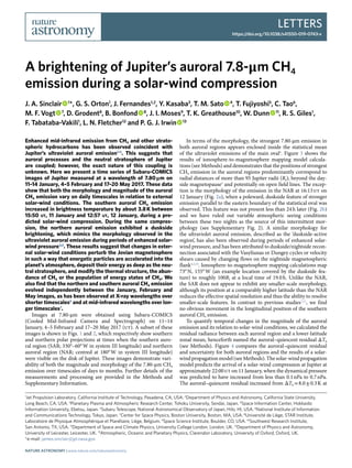
A brightening of Jupiter’s auroral 7.8-μm CH4 emission during a solar-wind compression

Enhanced mid-infrared emission from CH4 and other stratospheric hydrocarbons has been observed coincident with Jupiter’s ultraviolet auroral emission1–3 . This suggests that auroral processes and the neutral stratosphere of Jupiter are coupled; however, the exact nature of this coupling is unknown. Here we present a time series of Subaru-COMICS images of Jupiter measured at a wavelength of 7.80 μm on 11–14 January, 4–5 February and 17–20 May 2017. These data show that both the morphology and magnitude of the auroral CH4 emission vary on daily timescales in relation to external solar-wind conditions. The southern auroral CH4 emission increased in brightness temperature by about 3.8 K between 15:50 ut, 11 January and 12:57 ut, 12 January, during a predicted solar-wind compression. During the same compression, the northern auroral emission exhibited a duskside brightening, which mimics the morphology observed in the ultraviolet auroral emission during periods of enhanced solarwind pressure4,5 . These results suggest that changes in external solar-wind conditions perturb the Jovian magnetosphere in such a way that energetic particles are accelerated into the planet’s atmosphere, deposit their energy as deep as the neutral stratosphere, and modify the thermal structure, the abundance of CH4 or the population of energy states of CH4. We also find that the northern and southern auroral CH4 emission evolved independently between the January, February and May images, as has been observed at X-ray wavelengths over shorter timescales6 and at mid-infrared wavelengths over longer timescales7 .

Recommandé
Recommandé
Contenu connexe
Tendances
Tendances (20)
Similaire à A brightening of Jupiter’s auroral 7.8-μm CH4 emission during a solar-wind compression
Similaire à A brightening of Jupiter’s auroral 7.8-μm CH4 emission during a solar-wind compression (20)
Plus de Sérgio Sacani
Plus de Sérgio Sacani (20)
Dernier
Dernier (20)
A brightening of Jupiter’s auroral 7.8-μm CH4 emission during a solar-wind compression
- 1. Letters https://doi.org/10.1038/s41550-019-0743-x 1 Jet Propulsion Laboratory, California Institute of Technology, Pasadena, CA, USA. 2 Department of Physics and Astronomy, California State University, Long Beach, CA, USA. 3 Planetary Plasma and Atmospheric Research Center, Tohoku University, Sendai, Japan. 4 Space Information Center, Hokkaido Information University, Ebetsu, Japan. 5 Subaru Telescope, National Astronomical Observatory of Japan, Hilo, HI, USA. 6 National Institute of Information and Communications Technology, Tokyo, Japan. 7 Center for Space Physics, Boston University, Boston, MA, USA. 8 Université de Liège, STAR Institute, Laboratoire de Physique Atmosphérique et Planétaire, Liège, Belgium. 9 Space Science Institute, Boulder, CO, USA. 10 Southwest Research Institute, San Antonio, TX, USA. 11 Department of Space and Climate Physics, University College London, London, UK. 12 Department of Physics and Astronomy, University of Leicester, Leicester, UK. 13 Atmospheric, Oceanic and Planetary Physics, Clarendon Laboratory, University of Oxford, Oxford, UK. *e-mail: james.sinclair@jpl.nasa.gov Enhanced mid-infrared emission from CH4 and other strato- spheric hydrocarbons has been observed coincident with Jupiter’s ultraviolet auroral emission1–3 . This suggests that auroral processes and the neutral stratosphere of Jupiter are coupled; however, the exact nature of this coupling is unknown. Here we present a time series of Subaru-COMICS images of Jupiter measured at a wavelength of 7.80 μm on 11–14 January, 4–5 February and 17–20 May 2017. These data show that both the morphology and magnitude of the auroral CH4 emission vary on daily timescales in relation to external solar-wind conditions. The southern auroral CH4 emission increased in brightness temperature by about 3.8 K between 15:50 ut, 11 January and 12:57 ut, 12 January, during a pre- dicted solar-wind compression. During the same compres- sion, the northern auroral emission exhibited a duskside brightening, which mimics the morphology observed in the ultraviolet auroral emission during periods of enhanced solar- wind pressure4,5 . These results suggest that changes in exter- nal solar-wind conditions perturb the Jovian magnetosphere in such a way that energetic particles are accelerated into the planet’s atmosphere, deposit their energy as deep as the neu- tral stratosphere, and modify the thermal structure, the abun- dance of CH4 or the population of energy states of CH4. We also find that the northern and southern auroral CH4 emission evolved independently between the January, February and May images, as has been observed at X-ray wavelengths over shorter timescales6 and at mid-infrared wavelengths over lon- ger timescales7 . Images at 7.80-μm were obtained using Subaru-COMICS (Cooled Mid-Infrared Camera and Spectrograph) on 11–14 January, 4–5 February and 17–20 May 2017 (ut). A subset of these images is shown in Figs. 1 and 2, which respectively show southern and northern polar projections at times when the southern auro- ral region (SAR; 330°–60° W in system III longitude) and northern auroral region (NAR; centred at 180° W in system III longitude) were visible on the disk of Jupiter. These images demonstrate vari- ability of both the magnitude and morphology of the 7.80-μm CH4 emission over timescales of days to months. Further details of the measurements and processing are provided in the Methods and Supplementary Information. In terms of the morphology, the strongest 7.80-μm emission in both auroral regions appears enclosed inside the statistical mean of the ultraviolet emissions of the main oval8 . Figure 3 shows the results of ionosphere-to-magnetosphere mapping model calcula- tions (see Methods) and demonstrates that the positions of strongest CH4 emission in the auroral regions predominantly correspond to radial distances of more than 95 Jupiter radii (RJ); beyond the day- side magnetopause9 and potentially on open field lines. The excep- tion is the morphology of the emission in the NAR at 16:13 ut on 12 January (Fig. 2a), when a poleward, duskside feature of stronger emission parallel to the eastern boundary of the statistical oval was observed. This feature was not present less than 24 h later (Fig. 2b) and we have ruled out variable atmospheric seeing conditions between these two nights as the source of this intermittent mor- phology (see Supplementary Fig. 2). A similar morphology for the ultraviolet auroral emission, described as the ‘duskside-active region’, has also been observed during periods of enhanced solar- wind pressure, and has been attributed to duskside/nightside recon- nection associated with the Vasyliunas or Dungey cycles or velocity shears caused by changing flows on the nightside magnetospheric flank4,5,10 . Ionosphere-to-magnetosphere mapping calculations map 73° N, 155° W (an example location covered by the duskside fea- ture) to roughly 100RJ at a local time of 19.0 h. Unlike the NAR, the SAR does not appear to exhibit any smaller-scale morphology, although its position at a comparably higher latitude than the NAR reduces the effective spatial resolution and thus the ability to resolve smaller-scale features. In contrast to previous studies7,11 , we find no obvious movement in the longitudinal position of the southern auroral CH4 emission. To quantify temporal changes in the magnitude of the auroral emission and its relation to solar-wind conditions, we calculated the residual radiance between each auroral region and a lower-latitude zonal mean, henceforth named the auroral–quiescent residual ΔTb (see Methods). Figure 4 compares the auroral–quiescent residual and uncertainty for both auroral regions and the results of a solar- windpropagationmodel(seeMethods).Thesolar-windpropagation model predicts the arrival of a solar-wind compression at Jupiter at approximately 22:00 ut on 11 January, when the dynamical pressure was predicted to have increased from less than 0.1 nPa to 0.7 nPa. The auroral–quiescent residual increased from ΔTb = 8.0 ± 0.3 K at A brightening of Jupiter’s auroral 7.8-μm CH4 emission during a solar-wind compression J. A. Sinclair 1 *, G. S. Orton1 , J. Fernandes1,2 , Y. Kasaba3 , T. M. Sato 4 , T. Fujiyoshi5 , C. Tao6 , M. F. Vogt 7 , D. Grodent8 , B. Bonfond 8 , J. I. Moses9 , T. K. Greathouse10 , W. Dunn 11 , R. S. Giles1 , F. Tabataba-Vakili1 , L. N. Fletcher12 and P. G. J. Irwin 13 Nature Astronomy | www.nature.com/natureastronomy
- 2. Letters Nature Astronomy 15:50 ut 11 January to ΔTb = 11.8 ± 0.5 K at 12:57 ut 12 January—a net increase of 3.8 ± 0.6 K in brightness temperature Tb or a roughly 25% increase in radiance. Although the viewing geometries of the SAR differ between these two images, forward-model calculations of the 7.80-μm emission (see Methods) at these two geometries dif- fer by only 0.7 K in Tb and thus cannot explain all of the observed change. From 12:57 ut 12 January to 12:33 ut 14 January, the SAR returned to a brightness similar to that observed pre-compression; this brightness then remained roughly constant in all subsequent measurements (although variability between these measurements cannot be ruled out). The NAR was not visible on the disk of Jupiter in the images taken on 11 January (before the solar-wind compression) and so we do not know whether it also brightened during the same solar-wind com- pression. However, the aforementioned duskside-active emission captured by COMICS at 16:13 ut on 12 January (Fig. 2a) occurred shortly after the solar-wind compression, which reiterates that this morphology is probably driven by enhanced solar-wind conditions and their perturbing effect on the nightside magnetosphere. From 16:13 ut 12 January to 12:30 ut 13 January, the auroral–quiescent residual of the NAR was constant in time within uncertainty and subsequently decreased significantly to 1.2 ± 1.1 K. Similarly, mea- surements in May show the NAR emission to be weak and com- parable with, if not weaker than, lower-latitude regions. From 18 May to 19 May, there was a marginal increase in the emission in the NAR during a small solar-wind compression (about 0.2 nPa); however, the change in emission was not significant with respect to measurement uncertainty. Without measurements between 13 January, 5 February and 18 May, it is uncertain whether the NAR emission was consistently weaker in time or whether it exhib- ited short-term (daily or weekly) variability and the measurements by chance captured periods of weaker emission. We favour the latter possibility given that the measurements on 5 February and 17 May were preceded by at least seven days of steady, low-pressure (less than 0.05 nPa) solar-wind conditions. We note the results of a recent study12 , which showed that the total auroral power during a solar-wind compression exhibited a positive correlation with the duration of steady, quiescent solar-wind conditions preceding the compression. We also note that the northern auroral C2H6 emis- sion was shown in previous work to weaken during periods of low solar activity, which similarly suggests a connection with solar-wind conditions on longer timescales13 . 15:50 UT, 11 January 2017 300 300 300 60 60 60 –60 –60 –60 –45 12:57 UT, 12 January 2017 300 300 300 60 60 60 –75 –75 –75 –60 –60 –60 12:33 UT, 14 January 2017 –45 –45 14:58 UT, 4 Febuary 2017 09:40 UT, 17 May 2017 06:30 UT, 20 May 2017 140 145 150 155 160 Brightness temperature (K) –45 –45 –45 –75 –75 –75 a b e f c d Fig. 1 | Southern polar projections of Jupiter’s 7.80-μm CH4 emission. a–f, Images were recorded by Subaru-COMICS on 11 January (a), 12 January (b), 14 January (c), 4 February (d), 17 May (e) and 20 May (f) 2017. These are a subset of the observations shown in Supplementary Fig. 1, when the SAR (330°–60° W, system III) was fully or partially visible on the disk. The colour scale indicates the brightness temperature. Solid light-blue lines represent the statistical-mean position of the ultraviolet auroral main oval emission8 . For consistency with the Juno science team and the community supporting the Juno mission, increasing system III longitude is shown anticlockwise. All latitudes and longitudes are in degrees and are planetocentric and System III, respectively. Nature Astronomy | www.nature.com/natureastronomy
- 3. LettersNature Astronomy 16:13 UT, 12 January 2017 240 120 756045 12:30 UT, 13 January 2017 240 120 7560 15:54 UT, 5 Febuary 2017 240 120 756045 09:35 UT, 18 May 2017 240 120 7560 05:37 UT, 19 May 2017 240 120 756045 09:55 UT, 20 May 2017 240 120 7560 144 148 152 156 160 Brightness temperature (K) 45 45 45 a b c d e f Fig. 2 | Northern polar projections of Jupiter’s 7.80-μm CH4 emission. a–f, Images were recorded by Subaru-COMICS on 12 January (a), 13 January (b), 5 February (c) 18 May (d), 19 May (e) and 20 May (f) 2017. These are a subset of the observations shown in Supplementary Fig. 1, when the NAR (centred at 180° W, system III) was fully or partially visible on the disk. The colour scale indicates the brightness temperature. Solid light-blue lines represent the statistical- mean position of the ultraviolet auroral main oval emission8 . All latitudes and longitudes are in degrees and are planetocentric and System III, respectively. 75RJStatistical mean 55RJ Region A Region L 12:30 UT, 13 January 201712:57 UT, 12 January 2017 –75–60–45 –75–60–45 180 300 12024060 0 95RJ a b Fig. 3 | Polar projections and regions chosen for analysis. a,b, Subaru-COMICS 7.80-μm images recorded at 12:57 ut, 12 January 2017 (a; shown in the south) and 12:30 ut, 13 January 2017 (b; shown in the north), as in Figs. 1 and 2, shown again here for comparison with the ultraviolet main oval statistical mean8 and contours that map to different distances in the magnetosphere of Jupiter, as indicated in the legend. The region enclosed within the 95RJ contour is interpreted to map to the outer magnetosphere/magnetopause. Regions A and L (enclosed within the magenta and green regions) were chosen to represent the auroral and non-auroral regions, respectively, for calculations of the relative radiance and its variability, as detailed in the Methods. All latitudes and longitudes are in degrees and are planetocentric and System III, respectively. Nature Astronomy | www.nature.com/natureastronomy
- 4. Letters Nature Astronomy The daily variability of the southern auroral CH4 emission sug- gests that the source of the variability is in the upper stratosphere/ mesophere to thermosphere region (10–1 μbar), where the thermal inertial timescales are much shorter (around four weeks at 1 μbar)14 compared to the lower stratosphere (around 30 weeks at 1 mbar)14 . We suggest that the observed changes in CH4 emission result from: (1) variable auroral-related heating of the 10- to 1-μbar level, (2) auroral-driven changes in the vertical CH4 profile near its homo- pause at roughly 1 μbar, (3) variable non-local thermodynamic equilibrium (non-LTE) effects that modify the population of energy states of CH4 or (4) some combination of (1)–(3). To explore the first two possibilities and to determine what magnitude and type of change in the vertical temperature or CH4 profiles could yield an increase in Tb of 3–4 K at 7.80 μm, we performed a series of radia- tive-transfer calculations using NEMESIS (see Methods). As shown in Supplementary Fig. 5a,b, assuming the CH4 abun- dance is held fixed, a 3–4-K change in Tb would require either: (1) the pressure level of the mesosphere–thermosphere transition to move deeper in the atmosphere by approximately a pressure-scale height or (2) the lapse rate in the thermosphere to increase by a factor of 2. The former corresponds to a total, atmospheric tem- perature increase of more than 100 K at the 0.5-μbar level, assuming a thermospheric lapse rate similar to that measured during Galileo’s descent15 , whereas the latter corresponds to a total, atmospheric temperature increase of about 20 K at 0.5 μbar. In steady state, ther- mospheric general circulation models show that the mesosphere- to-thermosphere transition pressure is deeper in the auroral regions compared to the non-auroral regions16,17 . Yates et al.18 performed time-dependent thermospheric circulation modelling to investigate the response of the thermospheric structure and circulation to solar- wind compressions and expansion events. Between steady and com- pressed solar-wind conditions, the model predicted a warming of around 20 K and an increase in lapse rate near 70°N due to increased rates of joule heating at pressures lower than 1 μbar (with the lower model boundary set at 2 μbar). This is consistent with the two-fold increase of the thermospheric lapse rate required to brighten the 7.80-μm emission by 3–4 K, as detailed above. As shown in Supplementary Fig. 5c, assuming a fixed vertical temperature profile, increasing the altitude of the CH4 homopause (with respect to the Moses et al.19 model A CH4 profile) by greater than a pressure-scale height would yield a 3–4-K increase in Tb at 7.80 μm. At the 0.2-μbar level, this would correspond to an increase in the volume mixing ratio of the order of 10−4 . In solving the verti- cal continuity equation assuming that the change in volume mixing ratio is driven entirely by advection and not a chemical source (that is w = (−ΔX/Δt)/(ΔX/Δz), where w is the vertical velocity, X is the volume mixing ratio, t is time and z is height), a change in vertical wind of 2.7 cm s−1 with respect to the steady state would be required. The Bougher et al. thermospheric model16 predicts vertical winds near 70°S of approximately 50 cm s−1 at the 0.2-μbar level in steady state, and thus a change in vertical wind of 2.7 cm s−1 is reasonable. A higher-altitude homopause of CH4 (and other hydrocarbons) in Jupiter’s auroral regions was also found to optimize the consistency between Juno and Hisaki measurements20 . Non-LTE effects are likely to be important at the altitudes where the source of variability has been inferred or could itself be the driver of the observed variability. In the absence of a strong radiation source, classical non-LTE effects become non-negligible at pressures below 0.1 mbar, where collisional timescales become longer than the spontaneous radiative lifetime21–23 . Without a sufficient number of thermal collisions, the population of rotational and vibrational ener- gies deviates from the translational energy population and thus can no longer be described as a Boltzmann distribution. In comparison to non-auroral regions, the upper-stratospheric heating present in Jupiter’s auroral regions7,24,25 also yields a larger contribution of pho- tons at mid-infrared wavelengths from pressure levels where classi- cal non-LTE processes become non-negligible. In addition, currents of electrons and ions in Jupiter’s auroral regions and the resulting charged-particle collisions and dissociative recombinations may induce a non-Boltzmann population of the excited energy states of CH4. A further process might be ‘H3 + shine’, whereby the downward flux of H3 + emission in lines in the 3–4 μm range ‘pump’ overlapping CH4 ν3 lines, exciting the vibrational modes and thereby modifying the population of lines responsible for the ν4 band at approximately 7.80 μm (ref. 26 ). Modelling of the aforementioned non-LTE pro- cesses will be the subject of future work. We cannot distinguish between temperature, CH4 abundance and non-LTE effects driving the variable CH4 emission observed between 11 and 12 January 2017. Nevertheless, all of these processes describe a direct coupling of the neutral stratosphere in Jupiter’s auroral regions to the external magnetosphere of Jupiter and solar- wind environment. Although daily variability of the northern auroral C2H4 and C2H6 emission has been observed in previous studies27,28 , we believe that the results presented here represent a substantial advance in the understanding of this phenomenon. First, the availability of solar-wind measurements and their modelled propagation to Jupiter’s orbit allow the variability of the CH4 emis- sion to be tentatively linked to external solar-wind changes and their perturbing effect on the magnetosphere. Second, COMICS imaging at high-diffraction-limited spatial resolution allows the morphol- ogy of the CH4 emission and its variability to be resolved at finer spatial details and mapped to the outer magnetosphere/magneto- pause using ionosphere-to-magnetosphere mapping calculations. Auroral-related heating and chemistry dominate the forcing of the thermal structure and composition at Jupiter’s poles7,24,25 ; our results 5 Jan 10 Jan 15 Jan 20 Jan 25 Jan 30 Jan 4 Feb Date in 2017 0.0 0.2 0.4 0.6 0.8 Dynamicalpressure(nPa) South North –2 0 2 4 6 8 10 12 ΔTb(K) 5 May 10 May 15 May 20 May 25 May 30 May Date in 2017 0.0 0.2 0.4 0.6 0.8 Dynamicalpressure(nPa) South North –2 0 2 4 6 8 10 12 ΔTb(K) a b Fig. 4 | Auroral–quiescent residual over time. a,b, The residual 7.80-μm brightness temperature ΔTb (left axis) between region A and region L, as described in the text and Methods, are shown as red circles with error bars. Results are shown for January 2017 (a) and May 2017 (b). Predicted solar- wind dynamical pressure at Jupiter (right axis; see Methods) is shown as the solid black line, with horizontal error bars showing the potential time error. The data suggest a brightening of Jupiter’s southern auroral CH4 emission in response to a solar-wind compression at approximately 22:00 ut on 11 January 2017. Nature Astronomy | www.nature.com/natureastronomy
- 5. LettersNature Astronomy suggest that these processes are directly connected to the external magnetosphere. This phenomenon could therefore be ubiquitous for rapidly rotating Jupiter-like exoplanets with an internal plasma source around a magnetically active star29 . In particular, magnetohy- drodynamic simulations of a hot Jupiter at a close orbital separation of 0.05 au from its host star predict auroral powers several orders of magnitude larger than on Earth, affecting both polar and equato- rial regions30 . The coupling of the neutral stratosphere and magne- tosphere of Jupiter presented here may therefore be important in the near-future characterization of Jupiter-like exoplanets from the James Webb Space Telescope and of directly imaged planets whose atmospheres are sensed predominantly at higher latitudes. Methods COMICS 7.8-μm images. The COMICS31,32 instrument is mounted at the Cassegrain focus of the Subaru Telescope, which is located at the Mauna Kea Observatory (approximately 4.2 km above sea level). Subaru’s 8.2-m primary aperture provides a diffraction-limited spatial resolution of approximately 0.24″ at 7.8 μm, which corresponds to a latitude–longitude footprint of approximately 2.5° × 2° at ±70° latitude. COMICS provides both imaging and spectroscopic capabilities over a spectral range of approximately 7–25 μm. Images are measured on a 320 × 240 array of Si:As blocked impurity band pixels each with a scale of 0.13″, which provides a total field of view of 42″ × 32″. Images can be measured over a number of discrete filters in both the N band (7–13 μm) and Q band (17–25 μm). We focus on images obtained in the 7.80-μm filter, which is sensitive to Jupiter’s stratospheric CH4 emission (Supplementary Fig. 3). Images were measured on 11–14 January, 4–5 February and 17–20 May 2017. Measurements were performed during periods when Jupiter was available at airmasses lower than 3. The full disk of Jupiter (with equatorial diameters of approximately 36″ in January, 39″ in February and 42″ in May) could not be measured in a single image by the COMICS field of view. In the January and February measurements, the full disk of Jupiter was measured using a 2 × 1 mosaic of individual images centred at Jupiter’s mid-northern and mid-southern latitudes. In May, a 2 × 2 mosaic was conducted owing to Jupiter’s larger size during this time period. For each individual image, A-frames (of Jupiter) and B-frames (dark sky 60″ north of Jupiter) were continuously recorded over a total exposure time of 20 s. Further details of the measurements presented here are provided in Supplementary Table 1. Imaging processing, calibration and error handling. Images were processed and calibrated using the Data Reduction Manager. A −B subtraction was performed to remove telluric sky emission. The resulting images were then divided by a ‘bad pixel mask’ that accounts for corrupted pixels (due to cosmic ray damage, bright star saturation, manufacturer flaws, and so on) and by a flatfield to remove variations in pixel-to-pixel sensitivity across the detector. A limb-fitting procedure was used to assign latitudes, longitudes and local zenith angles to each pixel on the disk of Jupiter, using the known sub-observer latitude and longitudes at the time of each exposure. The absolute radiometric calibration of the images and correction for telluric absorption was conducted by scaling the observed lower-latitude zonal-mean brightness to those measured by Cassini’s CIRS33 instrument during the 2001 flyby. This procedure is described in greater detail in Fletcher et al.34 . We chose this method of calibration because experience with past mid-infrared images of Jupiter and Saturn has demonstrated that the radiometric calibration using a standard star provides inconsistency between datasets obtained on different nights34,35 . As detailed further in the Auroral–quiescent residual calculations section of Methods, our analysis of the images involved comparing the relative brightness of the auroral regions with a lower-latitude region over time, which negates errors introduced by offsets in the absolute calibration between nights. The reduced and radiometrically calibrated images are shown in Supplementary Fig. 1 in units of brightness temperature (Tb) at 7.80 μm. Portions of the image within 6 pixels (or approximately 0.8″) of the assigned limb were removed as a conservative means of removing the effects of seeing and diffraction in blurring dark sky together with emission from Jupiter. The noise-equivalent spectral radiance was calculated by finding the standard-deviation emission of dark-sky pixels more than 1.5″ (approximately 12 pixels) away from the planet. This was calculated for each image to capture changes in sensitivity due to variations in airmass and telluric atmospheric conditions between measurements. A centre-to- limb variation correction in the longitudinal direction was applied to correct for the foreshortening and limb-brightening, such that longitudes at different viewing geometries on different nights could be more readily compared. A power-law fit, of the form logR = alogμ + b, where R is radiance, μ = cosθ and θ is the zenith emission angle, was performed in each latitude band to derive a centre-to-limb correction factor. For the January and February measurements, we performed the power-law correction using the image from 15:50 ut 11 January (Supplementary Fig. 1a) in the northern hemisphere and the image from 12:30 ut 13 January (Supplementary Fig. 1d) in the southern hemisphere. For the May measurements, the images from 09:40 ut 17 May and 09:35 ut 18 May (Supplementary Fig. 1i,j) were similarly chosen to perform the power-law correction in the northern and southern hemispheres, respectively. These specific images were chosen because they best capture non-auroral longitudes in each hemisphere. Ionosphere-to-magnetosphere mapping. We adopted the ionosphere-to- magnetosphere mapping calculation by Vogt et al.36,37 to map a location on the planet in planetocentric latitude and system III longitude to its position in radial distance and local time in the Jovian magnetosphere. The calculation is performed by imposing magnetic flux equivalence of a specified region at the equator to the area at which it maps in the ionosphere assuming a given internal field model. We adopted the VIPAL (Voyager Io Pioneer Anomaly Longitude) internal field model38 owing to its validity in both the northern and southern hemispheres and to larger (roughly 95RJ) radial distances. Stepping through latitude and longitude in increments of 1° polewards of ±45° latitude, the ionosphere-to-magnetosphere mapping calculation was performed to derive the local time and distance within the magnetosphere at each location. Regions enclosed within the statistical ultraviolet oval for which the calculation did not produce a real value were interpreted as mapping beyond the 95RJ limit of the model, which also marks the estimated position of the dayside magnetopause9 . This calculation was used to derive the contours of distance shown in Fig. 3. Auroral–quiescent residual calculations. Figure 3 demonstrates the areas denoted by region A and region L at high northern and high southern latitudes. Region A was chosen as a subregion of the auroral regions that mapped to the outer magnetosphere and was commonly sampled by all measurements presented in Figs. 1 and 2. Region L was chosen as a lower-latitude region away from the area of auroral influence, which is sampled at μ = cos(θemm) (where θemm is the zenith emission angle on Jupiter) in the range 0.4 < μ < 1 in each image. By calculating the residual between region A and region L, any inconsistencies in the radiometric calibration from one night to the next are effectively removed, which would otherwise affect a comparison of the absolute radiance in time. The mean radiances within region A and region L were calculated. The 1σ uncertainty on the mean radiance in each region was chosen to be the larger of: (1) the noise-equivalent spectral radiance of each image (see the Imaging processing, calibration and error handling section of Methods) scaled by ∕ n1 p, where np is the number of pixels averaged, and (2) the standard deviation of the mean radiance in the region. The radiances and uncertainties were then converted to brightness-temperature units and the brightness-temperature residual and uncertainty were calculated. Solar-wind propagation model. The Juno spacecraft continues to provide information on the magnetic and charged-particle fields while performing 53.5-day orbits inside Jupiter’s magnetosphere. However, the Juno spacecraft cannot provide in situ measurements of the external solar-wind conditions outside Jupiter’s magnetosphere. In the absence of such measurements, we look to modelling results. A solar-wind propagation model39 was adopted to calculate the solar-wind dynamical pressure (pdyn = ρv2 , where ρ is the density and v is the velocity of the solar wind) impinging on Jupiter’s magnetosphere. This model is used extensively for the magnetospheres of the outer planets40–42 in the absence of in situ measurements of the solar-wind conditions. The model adopts hourly measurements of the solar wind and magnetic field at the nose of Earth’s bow shock from OMNI43 as input and then performs 1D magnetohydrodynamic (MHD) calculations to model the solar-wind flow out to Jupiter’s bow shock. The 1D model prediction of a 3D problem can introduce uncertainties on the arrival time and magnitude of the dynamical pressure of solar-wind compressions. When the magnitude of the Earth–Sun–Jupiter angle is less than 50°, the uncertainty of the arrival time of the solar-wind shock is less than ±20 h and that of the maximum dynamic pressure is 38% (ref. 12 ). Given the Earth–Sun–Jupiter angles were between 80° and 120° in during January–February 2017, we adopted a 48-h time error on the results of the solar-wind propagation model. In May 2017, the Earth–Sun–Jupiter angle was approximately 18° and thus we assumed a time error of 20 h for May 2017. These values also seem to be commensurate with a statistical comparison of 1D MHD predictions and solar-wind data measured by several spacecraft44 . These errors are shown in Fig. 4. Nemesis forward-model calculations. A single, broadband measurement of the CH4 emission does not provide sufficient information to invert or retrieve atmospheric parameters and determine at what altitudes they vary. Nevertheless, we computed synthetic or forward-model spectra for a range of vertical temperature and CH4 profiles to explore what changes in those atmospheric parameters could yield the observed 7.80-μm brightening of 3–4 K of the SAR. The NEMESIS forward model and retrieval tool45 was adopted to compute forward-model spectra of the radiance in the COMICS 7.80-μm bandpass. Forward-model spectra were computed using the line-by-line method using the sources of line information for CH4, CH3D and 13 CH4, C2H2, C2H6, NH3 and PH3 detailed in table 4 of Fletcher et al.46 . Calculations were performed using a square instrument function with a width of 0.04 cm−1 (chosen on the basis of a balance of a sufficiently high spectral resolution to resolve both weak and strong emission lines while minimizing computational expense) and subsequently convolved with the COMICS 7.80-μm bandpass and the telluric transmission spectrum Nature Astronomy | www.nature.com/natureastronomy
- 6. Letters Nature Astronomy (see Supplementary Fig. 2). The vertical temperature and CH4 profiles were varied as detailed below. The remaining parameters of our model atmosphere, including the vertical C2H2, C2H4, C2H6, NH3 and PH3 profiles, were held constant because they have negligible effect on the spectrum in the 7.80-μm bandpass. Further details of the model atmosphere are provided in Sinclair et al.24 . Note that the current NEMESIS forward model assumes LTE conditions, whereas conditions in the auroral regions may have departed from LTE, as discussed in the main text. First, we kept the vertical CH4 profile and its isotopologues fixed to the ‘model A’ vertical profile from Moses et al.19 . Starting from the temperature profile shown in Supplementary Fig. 4a, we modified the vertical temperature profile in the range 0.1 mbar to 1 μbar, which includes the transition from the upper stratosphere/mesosphere to the thermosphere. The vertical temperature gradient (or lapse rate) in thermosphere was fixed and the pressure level of the mesosphere–thermosphere transition was varied as shown in Supplementary Fig. 5a. For each profile, a forward model was computed at the same viewing angle (μ = cos(θemm) = 0.205) as region A in the SAR at 12:57 ut 12 January (during the solar-wind compression). The synthetic spectrum was convolved with the 7.80-μm bandpass (as detailed above) and converted to Tb. These Tb values are shown in the legend in Supplementary Fig. 5a. Further sets of forward models and brightness temperatures were similarly computed, where the pressure level of the mesosphere–thermosphere transition was fixed at 0.2 μbar and the vertical temperature gradient (or lapse rate) was varied, as shown in Supplementary Fig. 5b. Second, we fixed the vertical temperature profile as shown in Supplementary Fig. 4a. Starting from the vertical CH4 profile derived from model A of Moses et al.19 , the pressure level of the methane homopause was varied as shown in Supplementary Fig. 5c, and a forward-model radiance in the 7.80-μm bandpass was calculated and converted to Tb. These values are shown as the legend of Supplementary Fig. 5c. Data availability The COMICS images presented here are publicly available on the SMOKA (Subaru Mitaka Okayama-Kiso Archive) system (https://smoka.nao.ac.jp/). Reduced and calibrated images may be requested from J.A.S. The Data Reduction Manager is a suite of IDL software designed for reduction and processing of planetary images and is available in compressed format from G.S.O. on request (glenn.s.orton@jpl. nasa.gov). The ionosphere-to-magnetosphere mapping calculation is also written in IDL and is available from M.F.V. on request (mvogt@bu.edu). Results of the solar-wind propagation model in a specific time period may be requested from C.T. (chihiro.tao@nict.go.jp). The NEMESIS forward model and retrieval tool is written in Fortran and is available as a GitHub repository; a user account for this repository may be requested from P.G.J.I. (patrick.irwin@physics.ox.ac.uk). Received: 24 August 2018; Accepted: 4 March 2019; Published: xx xx xxxx References 1. Caldwell, J., Gillett, F. C. & Tokunaga, A. T. Possible infrared aurorae on Jupiter. Icarus 44, 667–675 (1980). 2. Kim, S. J., Caldwell, J., Rivolo, A. R., Wagener, R. & Orton, G. S. Infrared polar brightening on Jupiter. III. Spectrometry from the Voyager 1 IRIS experiment. Icarus 64, 233–248 (1985). 3. Flasar, F. M. et al. An intense stratospheric jet on Jupiter. Nature 427, 132–135 (2004). 4. Grodent, D., Gérard, J.-C., Clarke, J. T., Gladstone, G. R. & Waite, J. H. A possible auroral signature of a magnetotail reconnection process on Jupiter. J. Geophys. Res. Space 109, A05201 (2004). 5. Nichols, J. D. et al. Response of Jupiter’s auroras to conditions in the interplanetary medium as measured by the Hubble Space Telescope and Juno. Geophys. Res. Lett. 44, 7643–7652 (2017). 6. Dunn, W. R. et al. The independent pulsations of Jupiter’s northern and southern X-ray auroras. Nat. Astron. 1, 758–764 (2017). 7. Sinclair, J. A. et al. Independent evolution of stratospheric temperatures in Jupiter’s northern and southern auroral regions from 2014 to 2016. Geophys. Res. Lett. 44, 5345–5354 (2017). 8. Bonfond, B. et al. The tails of the satellite auroral footprints at Jupiter. J. Geophys. Res. Space 122, 7985–7996 (2017). 9. Joy, S. P. et al. Probabilistic models of the Jovian magnetopause and bow shock locations. J. Geophys. Res. Space 107, 1309 (2002). 10. Grodent, D. et al. Jupiter’s aurora observed with HST during Juno orbits 3 to 7. J. Geophys. Res. Space 123, 3299–3319 (2018). 11. Drossart, P. et al. Thermal profiles in the auroral regions of Jupiter. J. Geophys. Res. 98, 18803 (1993). 12. Kita, H. et al. Characteristics of solar wind control on Jovian UV auroral activity deciphered by long-term Hisaki EXCEED observations: evidence of preconditioning of the magnetosphere? Geophys. Res. Lett. 43, 6790–6798 (2016). 13. Kostiuk, T. et al. Variability of mid-infrared Aurora on Jupiter: 1979 to 2016. In American Geophysical Union Fall Meeting 2016 P33C-2155 (AGU, 2016). 14. Zhang, X. et al. Radiative forcing of the stratosphere of Jupiter, part I: atmospheric cooling rates from Voyager to Cassini. Planet. Space Sci. 88, 3–25 (2013). 15. Seiff, A. et al. Thermal structure of Jupiter’s atmosphere near the edge of a 5-μm hot spot in the north equatorial belt. J. Geophys. Res. 103, 22857–22890 (1998). 16. Bougher, S. W., Waite, J. H., Majeed, T. & Gladstone, G. R. Jupiter thermospheric general circulation model (JTGCM): global structure and dynamics driven by auroral and Joule heating. J. Geophys. Res. Planets 110, E04008 (2005). 17. Gérard, J.-C. et al. Altitude of Saturn’s aurora and its implications for the characteristic energy of precipitated electrons. Geophys. Res. Lett. 36, L02202 (2009). 18. Yates, J., Achilleos, N. & Guio, P. Response of the jovian thermosphere to a transient ‘pulse’ in solar wind pressure. Planet. Space Sci. 91, 27–44 (2014). 19. Moses, J. I. et al. Photochemistry and diffusion in Jupiter’s stratosphere: constraints from ISO observations and comparisons with other giant planets. J. Geophys. Res. Planets 110, E08001 (2005). 20. Clark, G. et al. Precipitating electron energy flux and characteristic energies in Jupiter’s main auroral region as measured by juno/jedi. J. Geophys. Res. Space 123, 7554–7567 (2018). 21. Appleby, J. F. CH4 nonlocal thermodynamic equilibrium in the atmospheres of the giant planets. Icarus 85, 355–379 (1990). 22. Kim, S. J. Infrared processes in the Jovian auroral zone. Icarus 75, 399–408 (1988). 23. López-Puertas, M. & Taylor, F. Non-LTE Radiative Transfer in the Atmosphere (World Scientific, 2001). 24. Sinclair, J. A. et al. Jupiter’s auroral-related stratospheric heating and chemistry I: analysis of Voyager-IRIS and Cassini-CIRS spectra. Icarus 292, 182–207 (2017). 25. Sinclair, J. A. et al. Jupiter’s auroral-related stratospheric heating and chemistry II: analysis of IRTF-TEXES spectra measured in December 2014. Icarus 300, 305–326 (2018). 26. Halthore, R. N., Allen, J. E. Jr & Decola, P. L. A non-LTE model for the Jovian methane infrared emissions at high spectral resolution. Astrophys. J. Lett. 424, L61–L64 (1994). 27. Kostiuk, T., Romani, P., Espenak, F. & Livengood, T. A. Temperature and abundances in the Jovian auroral stratosphere. 2: ethylene as a probe of the microbar region. J. Geophys. Res. 98, 18823 (1993). 28. Livengood, T. A., Kostiuk, T. & Espenak, F. Temperature and abundances in the Jovian auroral stratosphere. 1: ethane as a probe of the millibar region. J. Geophys. Res. 98, 18813 (1993). 29. Nichols, J. D. & Milan, S. E. Stellar wind-magnetosphere interaction at exoplanets: computations of auroral radio powers. Mon. Not. R. Astron. Soc. 461, 2353–2366 (2016). 30. Cohen, O., Kashyap, V. L., Drake, J. J., Sokolov, I. V. & Gombosi, T. I. The dynamics of stellar coronae harboring hot Jupiters. II. A space weather event on a hot Jupiter. Astrophys. J. 738, 166 (2011). 31. Kataza, H. et al. COMICS: the cooled mid-infrared camera and spectrometer for the Subaru telescope. Proc. SPIE 4008, 1144–1152 (2000). 32. Okamoto, Y. K. et al. Improved performances and capabilities of the cooled mid-infrared camera and spectrometer (COMICS) for the Subaru telescope. Proc. SPIE 4841, 169–180 (2003). 33. Flasar, F. M. et al. Exploring the Saturn system in the thermal infrared: the composite infrared spectrometer. Space Sci. Rev. 115, 169–297 (2004). 34. Fletcher, L. N. et al. Retrievals of atmospheric variables on the gas giants from ground-based mid-infrared imaging. Icarus 200, 154–175 (2009). 35. Parrish, P. D. et al. Saturn’s atmospheric structure: the intercomparison of Cassini/CIRS-derived temperatures with ground-based determinations. Bull. Am. Astron. Soc. 37, 680 (2005). 36. Vogt, M. F. et al. Improved mapping of Jupiter’s auroral features to magnetospheric sources. J. Geophys. Res. Space 116, A03220 (2011). 37. Vogt, M. F. et al. Magnetosphere-ionosphere mapping at Jupiter: quantifying the effects of using different internal field models. J. Geophys. Res. Space 120, 2584–2599 (2015). 38. Hess, S. L. G., Bonfond, B., Zarka, P. & Grodent, D. Model of the Jovian magnetic field topology constrained by the Io auroral emissions. J. Geophys. Res. Space 116, A05217 (2011). 39. Tao, C., Kataoka, R., Fukunishi, H., Takahashi, Y. & Yokoyama, T. Magnetic field variations in the jovian magnetotail induced by solar wind dynamic pressure enhancements. J. Geophys. Res. Space 110, A11208 (2005). 40. Badman, S. V. et al. Weakening of Jupiter’s main auroral emission during January 2014. Geophys. Res. Lett. 43, 988–997 (2016). 41. Kinrade, J. et al. An isolated, bright cusp aurora at Saturn. J. Geophys. Res. Space 122, 6121–6138 (2017). 42. Lamy, L. et al. The aurorae of Uranus past equinox. J. Geophys. Res. Space 122, 3997–4008 (2017). 43. Thatcher, L. J. & Müller, H.-R. Statistical investigation of hourly OMNI solar wind data. J. Geophys. Res. Space 116, A12107 (2011). Nature Astronomy | www.nature.com/natureastronomy
- 7. LettersNature Astronomy 44. Zieger, B. & Hansen, K. C. Statistical validation of a solar wind propagation model from 1 to 10 AU. J. Geophys. Res. Space 113, A08107 (2008). 45. Irwin, P. G. J. et al. The NEMESIS planetary atmosphere radiative transfer and retrieval tool. J. Quant. Spectrosc. Rad. Transfer 109, 1136–1150 (2008). 46. Fletcher, L. N. et al. The origin and evolution of Saturn’s 2011–2012 stratospheric vortex. Icarus 221, 560–586 (2012). Acknowledgements All data presented were obtained at the Subaru Telescope, which is operated by the National Astronomical Observatory of Japan. COMICS observations obtained on 11, 12 January and 19, 20 May were proposed by and awarded to Y.K. using Subaru classical time. COMICS observations on 13, 14 January, 4, 5 February and 17, 18 May were proposed by and awarded to G.S.O. through the Keck-Subaru time exchange programme. We acknowledge the W. M. Keck Observatory, which is operated as a scientific partnership between California Institute of Technology, the University of California and NASA and supported financially by the W. M. Keck Foundation. We recognize and acknowledge the very important cultural role and reverence that the summit of Maunakea has always had within the indigenous Hawaiian community. We are most fortunate to have the opportunity to conduct observations from this mountain. The research was carried out at the Jet Propulsion Laboratory, California Institute of Technology, under a contract with NASA. We thank the NASA Postdoctoral and Caltech programmes for funding and supporting J.A.S. during this research. G.S.O. was supported by grants from NASA to the Jet Propulsion Laboratory/California Institute of Technology. Author contributions J.A.S. led the analysis of the observations and the preparation of this Letter. G.S.O. and Y.K. were principal investigators of the awarded telescope time. J.A.S., G.S.O., Y.K., T.M.S. and T.F. participated in the measurements at the Subaru Telescope. J.F. performed the reduction and calibration of the images. C.T. and M.F.V. provided model output for the interpretation of the results. P.G.J.I. is the lead developer of the NEMESIS code. All remaining authors contributed to the interpretation of the results and the preparation of the Letter. Competing interests The authors declare no competing interests. Additional information Supplementary information is available for this paper at https://doi.org/10.1038/ s41550-019-0743-x. Reprints and permissions information is available at www.nature.com/reprints. Correspondence and requests for materials should be addressed to J.A.S. Publisher’s note: Springer Nature remains neutral with regard to jurisdictional claims in published maps and institutional affiliations. © The Author(s), under exclusive licence to Springer Nature Limited 2019 Nature Astronomy | www.nature.com/natureastronomy