1. LETTERS
PUBLISHED ONLINE: 22 JUNE 2014 | DOI: 10.1038/NGEO2190
Transient features in a Titan sea
J. D. Hofgartner1
*, A. G. Hayes1, J. I. Lunine1, H. Zebker2, B. W. Stiles3, C. Sotin3, J. W. Barnes4,
E. P. Turtle5, K. H. Baines3, R. H. Brown6, B. J. Buratti3, R. N. Clark7, P. Encrenaz8, R. D. Kirk9,
A. Le Gall10, R. M. Lopes3, R. D. Lorenz5, M. J. Malaska3, K. L. Mitchell3, P. D. Nicholson1, P. Paillou11,
J. Radebaugh12, S. D. Wall3 and C. Wood13
Titan’s surface–atmosphere system bears remarkable simi-
larities to Earth’s, the most striking being an active, global
methane cycle akin to Earth’s water cycle1,2
. Like the hydro-
logical cycle of Earth, Titan’s seasonal methane cycle is driven
by changes in the distribution of solar energy2
. The Cassini
spacecraft, which arrived at Saturn in 2004 in the midst of
northern winter and southern summer, has observed surface
changes, including shoreline recession, at Titan’s south pole3,4
and equator5
. However, active surface processes have yet to be
confirmed in the lakes and seas in Titan’s north polar region6–8
.
As the 2017 northern summer solstice approaches, the onset
of dynamic phenomena in this region is expected6,7,9–12
. Here
we present the discovery of bright features in recent Cassini
RADARdatathatappearedinTitan’snorthernsea,LigeiaMare,
in July 2013 and disappeared in subsequent observations.
We suggest that these bright features are best explained
by the occurrence of ephemeral phenomena such as surface
waves, rising bubbles, and suspended or floating solids. We
suggest that our observations are an initial glimpse of dynamic
processes that are commencing in the northern lakes and seas
as summer nears in the northern hemisphere.
Anomalous, bright features were detected in Titan’s north polar
sea, Ligeia Mare, by the Cassini Titan Radar Mapper13
(RADAR)
during the T92 synthetic aperture radar (SAR) pass (Fig. 1).
Three preceding SAR observations (T25, T29 and T64) and a
subsequent low-resolution SAR observation (T95) did not detect
the anomalous features. The faint, grey spots in the circle of the
T95 image are consistent with the speckle noise in the surrounding
sea region and thus are not anomalous. Radar backscatter above
the noise floor, however, was also detected during preceding T91
radar scatterometry-mode observations13
but we argue that this
signal may not have originated from the anomalies. Subsequent
Visual and Infrared Mapping Spectrometer (VIMS) and Imaging
Science Subsystem observations (T93 and T94) also did not detect
the anomalies. These eight passes, constituting all of the high-
resolution observations up to the present of the region of the
anomalous features, are shown in Fig. 1. In radar images, brightness
is determined by the normalized radar cross-section (NRCS), the
ratio of the radar energy backscattered to the receiver compared
with that from an isotropic scatterer14
. Dynamic processes such
as waves7
, suspended particles3
, or bubbles15
increase the NRCS.
Such phenomena have not been confirmed in Titan’s northern
lakes and seas, which have a dielectric constant that indicates a
methane–ethane composition and surface height variations of less
than 1 mm (ref. 8). The progressive seasonal increase in insolation
that is occurring however has been predicted to power the onset
of energetic processes6,7,9–12
and we argue that these anomalous
features are the observation of transient features in the seas. The
regional extent of the anomalous signal, which does not seem to
derive from a single contiguous structure but rather from distinct
features, is approximately 20 km by 20 km. A higher-zoom image of
the anomalous features is provided in the Supplementary Methods
along with further discussion of their morphology. The image
formed from the range/Doppler-processed, T91 scatterometry-
mode signal has noticeably more speckle and lower resolution than
the other images because scatterometry-mode observations are not
optimized for the formation of range/Doppler-processed images13
.
We argue that this image still contains credible signal despite the
greater speckle.
Hypotheses for the anomalous features detected in the T92
observation are organized into the following three broad categories.
Anomalies could arise from non-geophysical artefacts in the SAR
data, permanent, geophysical structures that are detected when
observed only with specific geometries, or transitory features that
are the result of a surface transformation. We systematically evaluate
each of these hypotheses in the following paragraphs.
The appearance of non-geophysical artefacts in SAR images is
a familiar problem in radar remote sensing and common artefacts
include ambiguities, scalloping, gain control, and edge effects14,16
.
Ambiguities result in a copy or ‘ghost’ of a region appearing offset
in the range and/or azimuth directions. Range ambiguities occur
when the radar instrument receives overlapping returns in the time
domain from adjacent echo pulses whereas azimuth ambiguities
arise from aliasing in the frequency domain of an echo. We found
that there are no structures that could have resulted in bright range
or azimuth ambiguities in the vicinity of the anomalous features.
Nadir ambiguities, scalloping, and gain control effects are unlikely to
create artefacts that are as spatially confined as the anomalies14
. The
anomalous features are surrounded by dark pixels, indicating that
they are unlikely the result of an edge effect. Thus, the anomalies
are not considered to be standard SAR image artefacts. We provide
more detailed arguments in the Supplementary Methods to support
our conclusion that a SAR artefact is not the explanation for the
anomalous features.
1Department of Astronomy, Cornell University, Ithaca, New York 14853, USA, 2Department of Electrical Engineering, Stanford University, Stanford,
California 94305-2215, USA, 3Jet Propulsion Laboratory, Pasadena, California 91109, USA, 4Department of Physics, University of Idaho, Moscow,
Idaho 83844-0903, USA, 5JHU Applied Physics Lab, Laurel, Maryland 20723, USA, 6Lunar and Planetary Laboratory, University of Arizona, Tucson,
Arizona 85721, USA, 7USGS Denver Federal Center, Denver, Colorado 80225-0046, USA, 8Observatoire de Paris, Paris 75014, France, 9USGS
Astrogeology Center, Flagstaff, Arizona 86001, USA, 10LATMOS-UVSQ, Paris 78280, France, 11University of Bordeaux, Bordeaux 33271, France,
12Department of Geological Sciences, Brigham Young University, Provo, Utah 84602, USA, 13Planetary Science Institute, Tucson, Arizona 85721, USA.
*e-mail: jhofgartner@astro.cornell.edu
NATURE GEOSCIENCE | ADVANCE ONLINE PUBLICATION | www.nature.com/naturegeoscience 1
© 2014 Macmillan Publishers Limited. All rights reserved.

2. LETTERS NATURE GEOSCIENCE DOI: 10.1038/NGEO2190
150° E135° E120° E105° E90° E75° E
80°N75°N
T25 SAR
02/22/2007
i = 20°
SAR mosaic of
Ligeia Mare
T29 SAR
i = 19°
T91 range/
Doppler scatterometry
05/23/2013
T64 SAR
i = 36°
T92 SAR
i = 6°
07/10/2013
Anomalous
features
T94 VIMS 09/12/2013 T95 low-resolution SAR
10/14/2013
i = 27°
T93 VIMS 07/26/2013
0 50 100 150 20025
km
0 10 20 30
km
04/26/2007 12/27/2009
i = 3°
Figure 1 | Titan’s Ligeia Mare and high-resolution Cassini observations of the region of the anomalous features (green outlines). In the T92 image,
anomalous, bright features (circled in red) are observed at 78◦ N, 123◦ E that are not seen in any of the other SAR or VIMS images. Similarly sized, nearby
peninsulas (bright region at the bottom right), however, were consistently detected. The transient anomalies were probably not present during the T91
scatterometry-mode observation. Pixel brightness is linearly related to normalized radar cross-section. Green rectangle indicates the extent of the
high-resolution images, and green ovals correspond to the area circled in red. White arrows in radar images indicate the radar illumination direction. The
blue line indicates the transect for Fig. 3.
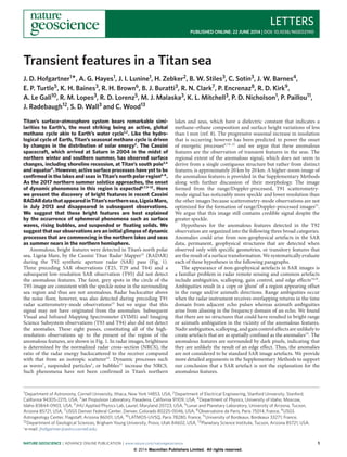
For Cassini RADAR measurements of a permanent, geophysical
structure on Titan, the angle of incidence is the dominant
geometrical parameter for the measured NRCS. These two variables
are inversely correlated; that is, increasing the angle of incidence
decreases the NRCS (ref. 14). Figure 2 is a plot of the NRCS from
the region of the anomalous features as a function of incidence
angle. Only the T91 and T92 observations, at incidence angles of
3 and 6 degrees respectively from the surface normal (black circles),
measured radar backscatter above the noise floor (red triangles).
Thus, any model for the anomalous features as permanent, static
2 NATURE GEOSCIENCE | ADVANCE ONLINE PUBLICATION | www.nature.com/naturegeoscience
© 2014 Macmillan Publishers Limited. All rights reserved.

3. NATURE GEOSCIENCE DOI: 10.1038/NGEO2190 LETTERS
0 5 10 15 20 25 30 35 40
−25
−20
−15
−10
−5
0
5
Incidence angle (°)
Normalizedradarcross-section(dB)
T64
T95
T25
T29
T91
T92
Mean of the anomalous features
Mean noise floor
Best-fit Hagfors model ( = 5.5°, = 2.0)
Nearby peninsula
α
Best-fit exponential model ( = 11.7°, = 1.9)
Best-fit Gaussian model ( = 11.1°, = 1.9)
α ε
α ε
ε
Figure 2 | Normalized radar cross-section of the region of the anomalous
features as a function of incidence angle. Only the T91 and T92
observations, at incidence angles of 3.4 and 6.0 degrees respectively (black
circles), measured radar backscatter above the noise floor (red triangles).
Quasi-specular models are ruled out to 88% confidence because, as
shown, most cannot simultaneously satisfy the shallow slope between the
T91 and T92 observations and the upper limits at higher incidence angles.
The grey shaded region shows the behaviour of the nearby peninsulas,
which is consistent with quasi-specular plus diffuse scattering. Error bars
show one-sigma confidence.
structures must be consistent with the T91 and T92 measurements
and stay below the noise floor values of the higher incidence angle
observations (otherwise the anomalous features would have been
detected in those observations as well). Empirically, all terrains
on Titan can be well fitted by combined quasi-specular and
diffuse backscatter models17,18
, including the nearby peninsulas
(Supplementary Methods), visible towards the lower right in the
zoom panels of Fig. 1. We compared the observations of the
anomalies with a suite of quasi-specular plus diffuse backscatter
models and found that this class of models for a permanent structure
can be ruled out to 88% confidence (Methods). The best-fit models
are plotted in Fig. 2 and their parameters are given in the legend. We
also considered models for submerged seamounts, using constraints
for the surface roughness and dielectric constant of Ligeia Mare
derived from recent analyses of the nadir (0 degrees incidence)
signal in the T91 observation8,19
and found that these models are
also ruled out to 88% confidence (Methods). We note that it is the
combination of the small likelihood that the NRCS at 3 degrees is
larger than at 6 degrees with the low upper limits at higher incidence
angles that inhibits the models from fitting the observations.
We point out that the NRCS upper limits for incidence angles
of greater than 15 degrees require that permanent models for
the anomalous features not exhibit any appreciable diffuse radar
scattering. An absence of diffuse radar scattering however is
discordant with the general conclusion, not only from the Cassini
spacecraft’s 2.2 cm wavelength observations but also from the
3.5 cm and 12.6 cm Earth-based observations, that radar scattering
on Titan is dominated by diffuse backscatter17,18,20,21
. The nearby
peninsulas, for example, exhibit significant diffuse backscatter, as
shown by the grey shaded region in Fig. 2. Thus, the set of models
that has a 12% chance of corresponding to the data has the important
caveat that none of those models scatters radar waves diffusely,
a behaviour that is dissimilar from all other terrains on Titan.
Therefore, we also consider those models implausible.
The T91 and T92 NRCS profiles along a transect of Titan that
crosses Ligeia Mare and includes the region of the anomalous
0 25 50 75 100 125 150 175 200 225
−30
−25
−20
−15
−10
−5
0
5
10
15
Along-track distance (km)
Normalizedradarcross-section(dB)
T91
T92
Noise floors
Sea
Figure 3 | Normalized radar cross-section profiles along a transect of
Titan that crosses Ligeia Mare including the region of the anomalous
features. The correlation of the profiles suggests that the signal in the T91
image is valid. At the anomalous features (green oval), the T92 profile
exhibits a large spike but no similar spike is observed in the T91 profile.
Incidence angle increases from 3.3◦–3.5◦ and 4.6◦–6.2◦ for the T91 and T92
observations respectively. The blue line in Fig. 1 indicates the centre of the
transect. The error bars show the one-sigma confidence.
features are plotted in Fig. 3. These profiles, which are both above
their respective noise floors, are correlated and the lesser T92
NRCS, relative to that of T91, is due to its greater incidence
angle. This behaviour is consistent, for example, with the radar
transmitting through the liquid and scattering off the seabed as
claimed by other analyses3,19,22,23
. In the region of the anomalies,
however, the T92 profile exhibits a large spike in NRCS but no
similar anomalous spike is observed in the T91 profile. Therefore,
we conclude that the anomalous features were not present at the time
of the T91 observation.
Transitory hypotheses envisage that a transformation occurred
before the discovery of the anomalous features and that their
detection thus depends primarily on the timing of the observation.
The anomalies were not detected in three observations before 2013,
were detected in the T92 observation on 10 July 2013 and then not
detected in three subsequent observations (Fig. 1). A signal was
detected in the T91 observation on 23 May 2013 but as previously
discussed, the transient anomalies probably were not present during
this observation. Therefore, the evolution of the anomalous features
seems to have included a reversion after the T92 pass and we do
not consider further hypotheses that predict the formation of a
new permanent structure, such as an island through cryovolcanism
and restrict further discussion to hypotheses for ephemeral features.
From recent analysis of the nadir signal in the T91 observation19
,
the absorption of the radar energy as it propagates through the sea
is constrained to be small. Thus, variations in sea level should not
strongly influence the measured NRCS and are unlikely to explain
the transient anomalies. With the exception of the T25 and T29
passes, all of the passes occurred at the same true orbital anomaly
and thus hypotheses that depend on Titan’s orbit around Saturn,
such as tides, are also not considered further.
The remaining transient hypotheses include waves, rising
bubbles, and suspended and/or floating solids. The data do
not permit us to further discard any of these hypotheses with
confidence. Titan’s northern hemisphere is transitioning from
vernal equinox (August 2009) to summer solstice (May 2017) and it
is plausible that the anomalous, transient features are an expression
NATURE GEOSCIENCE | ADVANCE ONLINE PUBLICATION | www.nature.com/naturegeoscience 3
© 2014 Macmillan Publishers Limited. All rights reserved.

4. LETTERS NATURE GEOSCIENCE DOI: 10.1038/NGEO2190
of the changing seasons. Waves were/are expected to form and
become detectable as wind speeds in the northern hemisphere climb
with the approach of summer6,7,9,10
. Thermal perturbations could
lead to the exsolution of gases from the liquid and/or sea floor
that form bubbles and buoyantly rise to the surface. Polyacetylene
and other low-density solids could be suspended in the sea24
much like silt in a terrestrial delta (backscatter variation, possibly
from a transient surface layer with distinct dielectric properties,
has been previously observed near an estuary of Kraken Mare3
)
and it has been predicted that sunken solids formed from a
winter freeze could become buoyant with the onset of warmer
temperatures12
. This discussion of seasonal mechanisms is not
inclusive and all of the remaining hypotheses may have additional
plausible mechanisms.
Some of the ephemeral phenomena cited above as causes of the
transient radar signature may be stimulated or enhanced by regional
meteorological phenomena, such as wind or rain. Although Cassini
did not detect any clouds during the T92 pass, the geometry was
rather unfavourable for detection above the site of the anomalies;
we note, however, that during the T93 pass VIMS detected a cloud,
approximately 100 km in diameter, about 350 km from the region of
the transients.
Methods
Mask. To determine the mean NRCS of the regions of the anomalous features
and thus produce the plot in Fig. 2, it was necessary to define a mask that
encompassed exclusively the regions of the anomalous features. We considered a
zone that, from visual inspection, included all pixels of the anomalous features as
well as some sea pixels but none of the shore. The mask for the anomalies was
defined as all pixels in this zone with an NRCS in the T92 image of greater than
0.25 and was used to determine the average characteristics in each observation of
the region of the anomalies. The cutoff of 0.25 was selected to eliminate >99% of
the sea pixels, from analysis of their backscatter distribution, but retain most of
the pixels of the anomalous features. As radar measurements of any feature will
have an exponential distribution (speckle), a threshold that removes the lower
end of the distribution biases the mean NRCS towards a higher value. We found
that the cutoff only minimally biased the T92 NRCS and did not significantly
affect the results.
Modelling. We considered three classes of quasi-specular models: exponential,
Gaussian and Hagfors18
. To test whether the data are consistent with these
models, we simulated the T91 and T92 observations by randomly generating
NRCS values such that they followed a normal distribution, with the mean and
standard deviation given by the observed NRCS and error. We then checked
whether any models fit the two simulated backscatter measurements and
remained below the upper limits at higher incidence angles. The exponential,
Gaussian and Hagfors models failed to fit the data in >99%, 88% and >99% of
the simulations respectively. The best-fit models are plotted in Fig. 2 and their
root-mean-square roughnesses and effective dielectric constants are given in the
legend. The success rate of Gaussian models was greater than exponential and
Hagfors models because they predict a shallower gradient in NRCS at the lowest
incidence angles (less than about 10 degrees) and a steeper gradient at higher
incidence angles. This is consistent with the measured NRCS, which is
approximately flat for the lowest incidence angles but significantly reduced by
about 20 degrees incidence.
Including the additional physics of refraction and loss due to reflection at the
atmosphere–sea interface23
, we followed the same prescription as above to test
models for submerged seamounts. We used the recently measured index of
refraction for Ligeia Mare to calculate the refracted incidence angles of the
radar19
and considered a perfectly flat surface for Ligeia Mare, consistent with
recent measurements8
, when calculating the Fresnel transmission coefficients.
Received 13 March 2014; accepted 20 May 2014;
published online 22 June 2014
References
1. Atreya, S. K. et al. Titan’s methane cycle. Planet. Space Sci. 54,
1177–1187 (2006).
2. Lunine, J. I. & Atreya, S. K. The methane cycle on Titan. Nature Geosci. 1,
159–164 (2008).
3. Hayes, A. G. et al. Transient surface liquid in Titan’s polar regions from Cassini.
Icarus 211, 655–671 (2011).
4. Turtle, E. P., Perry, J. E., Hayes, A. G. & McEwen, A. S. Shoreline retreat at
Titan’s Ontario Lacus and Arrakis Planitia from Cassini Imaging Science
Subsystem observations. Icarus 212, 957–959 (2011).
5. Turtle, E. P. et al. Rapid and extensive surface changes near Titan’s equator:
Evidence of April showers. Science 331, 1414–1417 (2011).
6. Lorenz, R. D., Newman, C. & Lunine, J. I. Threshold of wave generation on
Titan’s lakes and seas: Effect of viscosity and implications for Cassini
observations. Icarus 207, 932–937 (2010).
7. Hayes, A. G. et al. Wind driven capillary-gravity waves on Titan’s lakes: Hard to
detect or non-existent? Icarus 225, 403–412 (2013).
8. Zebker, H. A. et al. Surface of Ligeia Mare, Titan, from Cassini altimeter and
radiometer analysis. Geophys. Res. Lett. 41, 308–313 (2013).
9. Tokano, T. Limnological structure of Titan’s hydrocarbon lakes and its
astrobiological implication. Astrobiology 9, 147–164 (2009).
10. Tokano, T. Are tropical cyclones possible over Titan’s seas? Icarus 223,
766–774 (2013).
11. Roe, H. G. & Grundy, W.M. Buoyancy of ice in the CH4–N2 system. Icarus 219,
733–736 (2012).
12. Hofgartner, J. D. & Lunine, J. I. Does ice float in Titan’s lakes and seas? Icarus
223, 628–631 (2013).
13. Elachi, C. et al. RADAR: The Cassini Titan radar mapper. Space Sci. Rev. 115,
71–110 (2004).
14. Elachi, C. & van Zyl, J. Introduction to the Physics and Techniques of Remote
Sensing (Wiley, 2006).
15. Engram, M., Anthony, K. W., Meyer, F. J. & Grosse, G. Synthetic aperture radar
(SAR) backscatter response from methane ebullition bubbles trapped by
thermokarst lake ice. Can. J. Remote Sens. 38, 667–682 (2012).
16. Stiles, B. W. et al. Ground processing of Cassini RADAR imagery of Titan.
(Proc. IEEE Conference on RADAR, 2006).
17. Wye, L. C. et al. Electrical properties of Titan’s surface from Cassini RADAR
scatterometer measurements. Icarus 188, 367–385 (2007).
18. Wye, L. C. Radar scattering from Titan and Saturn’s icy satellites using the
Cassini spacecraft. PhD thesis, Stanford University, Faculty of Engineering,
316 (2011).
19. Mastroguiseppe, M. et al. The bathymetry of a Titan sea. Geophys. Res. Lett. 41,
1432–1437 (2014).
20. Muhleman, D. O., Grossman, A. W. & Butler, B. J. Radar investigations of Mars,
Mercury, and Titan. Annu. Rev. Earth Planet. Sci. 23, 337–374 (1995).
21. Campbell, D. B., Black, G. J., Carter, L. M. & Ostro, S. J. Radar evidence for
liquid surfaces on Titan. Science 302, 431–434 (2003).
22. Hayes, A. G. et al. Hydrocarbon lakes on Titan: Distribution and interaction
with a porous regolith. Geophys. Res. Lett. 35, L09204 (2008).
23. Hayes, A. G. et al. Bathymetry and absorptivity of Titan’s Ontario Lacus.
J. Geophys. Res. 115, E09009 (2010).
24. Chien, J. C. W. Polyacetylene Chemistry, Physics and Material Science (Academic
Press, 1984).
Acknowledgements
J.D.H. gratefully acknowledges the Cassini RADAR and VIMS Teams for the data
and the opportunity to lead the analysis and the Cassini Project and Natural Sciences
and Engineering Research Council of Canada, Post Graduate Scholarship Program for
financial support. A.G.H. was partially supported by NASA grant NNX13AG03G.
A portion of this work was performed at the Jet Propulsion Laboratory, California
Institute of Technology under a contract with the National Aeronautics and
Space Administration.
Author contributions
J.D.H. led the analysis and writing of the letter. A.G.H. and J.I.L. worked closely with
J.D.H. on all aspects of the analysis and writing. H.Z. worked closely with J.D.H. on the
NRCS analysis. B.W.S. contributed the SAR processing and artefact analysis and that
section of the letter. C.S., J.W.B. and E.P.T. contributed to the VIMS and Imaging
Science Subsystem analysis and the cloud discussion. All authors contributed to the
data acquisition and discussions.
Additional information
Supplementary information is available in the online version of the paper. Reprints and
permissions information is available online at www.nature.com/reprints.
Correspondence and requests for materials should be addressed to J.D.H.
Competing financial interests
The authors declare no competing financial interests.
4 NATURE GEOSCIENCE | ADVANCE ONLINE PUBLICATION | www.nature.com/naturegeoscience
© 2014 Macmillan Publishers Limited. All rights reserved.