1. VoIP and Multimedia Networking
Overview of IP Telephony
An IP telephone can be used to make telephone calls over IP networks. Voice
over IP (VoIP), or IP telephony, uses packet-switched networks to carry voice traffic in
addition to data traffic. The basic scheme of IP telephony starts with pulse code
modulation.
The encoded data is transmitted as packets over packet-switched networks. At a
receiver, the data is decoded and converted back to analog form. The packet size must be
properly chosen to prevent large delays. The IP telephone system must also be able to
handle the signaling function of the call setup, mapping of phone number to IP address,
and proper call termination.
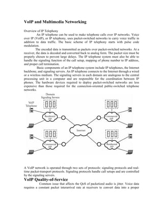
Basic components of an IP telephone system include IP telephones, the Internet
backbone, and signaling servers. An IP telephone connects to the Internet through a wired
or a wireless medium. The signaling servers in each domain are analogous to the central
processing unit in a computer and are responsible for the coordination between IP
phones. The hardware devices required to deploy packet-switched networks are less
expensive than those required for the connection-oriented public-switched telephone
networks.
A VoIP network is operated through two sets of protocols: signaling protocols and real-
time packet-transport protocols. Signaling protocols handle call setups and are controlled
by the signaling servers.
VoIP Quality-of-Service
Common issue that affects the QoS of packetized audio is jitter. Voice data
requires a constant packet interarrival rate at receivers to convert data into a proper

2. analog signal for playback. The variations in the packet interarrival rate lead to jitter,
which results in improper signal reconstruction at the receiver. Typically, an unstable sine
wave reproduced at the receiver results from the jitter in the signal.
A VoIP connection has several QoS factors:
• Packet loss is accepted to a certain extent.
• Packet delay is normally unacceptable.
• Jitter, as the variation in packet arrival time, is not acceptable after a certain limit.
Packet loss is a direct result of the queuing scheme used in routers. VoIP can use priority
queuing, weighted fair queuing, or class-based weighted fair queuing, whereby traffic
amounts are also assigned to classes of data traffic. Besides these well-known queuing
schemes, voice traffic can be handled by a custom queuing, in which a certain amount of
channel bandwidth for voice traffic is reserved.
VoIP Signaling Protocols
The IP telephone system must be able to handle signaling for call
setup, conversion of phone number to IP address mapping, and proper call termination.
IP telephone systems can use either a distributed or a centralized
signaling scheme. The distributed approach enables two IP telephones to communicate
using a client/ server model, as most Internet applications do. The distributed approach
works well with VoIP networks within a single company. The centralized approach uses
the conventional model and can provide some level of guarantee. Three well-known
signaling protocols are
1. Session Initiation Protocol (SIP)
2. H.323 protocols
3. Media Gateway Control Protocol (MGCP)

3. Session Initiation Protocol (SIP)
The Session Initiation Protocol (SIP) is one of the most important VoIP signaling
protocols operating in the application layer in the five-layer TCP/IP model. SIP can
perform both unicast and multicast sessions and supports user mobility. SIP handles
signals and identifies user location, call setup, call termination, and busy signals. SIP can
use multicast to support conference calls and uses the Session Description Protocol (SDP)
to negotiate parameters.
SIP Components
The following figure shows the SIP protocol.call is initiated from a user agent: the user's
IP telephone system, which is similar to a conventional phone. A user agent
assists in initiating or terminating a phone call in VoIP networks. A user agent
can be implemented in a standard telephone or in a laptop with a microphone
that runs some software. A user agent is identified using its associated domain.
For example, user1@domain1.com refers to user 1, who is associated with the
domain1.com network.
SIP consists of the following five servers
1. DNS server
2. Proxy server.
3. Location server.
4. Redirect server.
5. Registrar server.
Session Signaling and Numbering
Following Figure shows a SIP session between user agents 1 and 2:
user1@domain1.com and user2@domain2.com, respectively. In this example,
user 1 places a call to contact user 2. User 1 first communicates with its DNS
server to map the domain name to an IP address in the SIP UID. The DNS
server then communicates with the proxy server of the called party. At this

4. point, user 1 has resolved the name of user2@domain2.com into an IP address
through DNS query and response.

5. The first signal to establish this call is the INVITE message, which is used for session
creation. The INVITE message contains such information fields as from, to,
via, and call-id, in addition to routing information.
H.323 Protocols
The H.323-series protocols are implemented in layer 5 of the TCP/IP model and run over
either TCP or UDP. The H.323 protocols interact to provide ideal telephone
communication, providing phone numbers to IP address mapping, handling
digitized audio streaming in IP telephony, and providing signaling functions
for call setup and call management.
H.323 Components
. The H.323 scheme defines the following five components:
1. Multimedia terminal. A multimedia terminal is designed to support video and data
traffic and to provide support for IP telephony.
2. DNS server. As in SIP, a DNS server maps a domain name to an IP address.
3. Gateway. The gateway is a router that serves as an interface between the IP
telephone system and the traditional telephone network.

6. 4. Gatekeeper: The gatekeeper is the control center that performs all the location and
signaling functions. The gatekeeper monitors and coordinates the activities of the
gateway. The gateway also performs some signaling functions.
5. Multicast or multipoint control unit (MCU). This unit provides some multipoint
services, such as conference calls.
Session Signaling and Numbering

7. First, user 1 communicates with its DNS server, as explained earlier. The signaling uses
both UDP and TCP, and partitioned into the following five steps:
1. Call setup
2. Initial communication capability
3. Audio/video communication establishment
4. Communications
5. Call termination
At step 1, when user1 dials user 2's telephone number, the first set of signals are
exchanged between these two users in conjunction with opening a TCP connection. TCP-
SYN, TCP-SYN-ACK, and then TCP-ACK signals are generated between the two users.
At this point, the H225.0 SETUP ON TCP signal informs the called party that the
connection can be set up on TCP. The users can now request a certain bandwidth from
the associated gatekeeper server of the called party.
Real-Time Media Transport Protocols
In real-time applications, a stream of data is sent at a constant rate. This data must be
delivered to the appropriate application on the destination system, using real-time
protocols. The most widely applied protocol for real-time transmission is the Real-Time
Transport Protocol (RTP), including its companion version: Real-Time Control Protocol
(RTCP).
Real-Time Transport Protocol (RTP)
The real-time transport protocol (RTP) provides some basic functionalities to
real-time applications and includes some specific functions to each application. RTP runs
on top of the transport protocol as UDP.
Real-time applications, such as voice and video, can tolerate a certain amount of
packet loss and do not always require data retransmission. The mechanism RTP uses
typically informs a source about the quality of delivery. The source then adapts its
sending rate accordingly. If the rate of packet loss is very high, the source might switch to
a lower-quality transmission, thereby placing less load on the network.
Real-Time Session and Data Transfer
The TCP/IP and OSI models divide the network functionalities, based on a layered
architecture. Each layer performs distinct functions, and the data flows sequentially
between layers. The layered architecture may restrict the implementation on certain
functions out of the layered order. Integrated layer processing dictates a tighter coupling
among layers. RTP is used to transfer data among sessions in real time. A session is a
logical connection between an active client and an active server and is defined by the
following entities:

8. • RTP port number, which represents the destination port address of the RTP
session. Since RTP runs over UDP, the destination port address is available on the
UDP header.
• IP address of the RTP entity, which involves an RTP session. This address can be
either a unicast or a multicast address.
RTP Packet Header
The RTP header fields are:
• Version (V), a 2-bit field indicating the protocol version.
• Padding (P), a 1-bit field that indicates the existence of a padding field at the end
of the payload. Padding is required in applications that require the payload to be a
multiple of some length.
• Extension (X), a 1-bit field indicating the use of an extension header for RTP.
• Contributing source count (CSC), a 4-bit field that indicates the number of
contributing source identifiers.
• Marker (M), a 1-bit field indicating boundaries in a stream of data traffic. For
video applications, this field can be used to indicate the end of a frame.
• Payload type, A 7-bit field specifying the type of RTP payload. This field also
contains information on the use of compression or encryption.
• Sequence number, a 16-bit field that a sender uses to identify a particular packet
within a sequence of packets. This field is used to detect packet loss and for
packet reordering.
• Timestamp, a 32-bit field enabling the receiver to recover timing information.
This field indicates the timestamp when the first byte of data in the payload was
generated.
• Synchronization source identifier, a randomly generated field used to identify the
RTP source in an RTP session.
• Contributing source identifier, an optional field in the header to indicate the
contributing sources for the data.
Real-Time Control Protocol (RTCP)
The Real-Time Transport Protocol (RTCP) also runs on top of UDP. RTCP
performs several functions, using multicasting to provide feedback about the data quality

9. to all session members. The session multicast members can thus get an estimate of the
performance of other members in the current active session. Senders can send reports
about data rates and the quality of data transmission.
Packet Type and Format
The fields in the sender information block are:
• NTP timestamp, a 64-bit field that indicates when a sender report was sent. The
sender can use this field in combination with the timestamp field returned in
receiver reports to estimate the round-trip delay to receivers.
• RTP timestamp, a 32-bit field used by a receiver to sequence RTP data packets
from a particular source.
• Sender's packet count, a 32-bit field that represents the number of RTP data
packets transmitted by the sender in the current session.
• Sender's byte count, a 32-bit field that represents the number of RTP data octets
transmitted by the sender in the current session.
The SR packet includes zeros or more RR blocks. One receiver block is included for each
sender from which the member has received data during the session. The RR block
includes the following fields:
• SSRC_n, a 32-bit field that identifies the source in the report block, where n is the
number of sources.
• Fraction lost, an 8-bit field indicating the fraction of data packet loss from source
SSRC_n since the last SR or RR report was sent.

10. • Cumulative number of packets lost, a 24-bit field that represents the total number
of RTP data packets lost from the source in the current active session identified by
SSRC_n.
• Extended highest sequence number received, the first 16 least-significant bits,
used to indicate the highest sequence number for packets received from source
SSRC_n. The first 16 most-significant bits indicate the number of times that the
sequence number has been wrapped back to zero.
• Interarrival jitter, a 32-bit field used to indicate the jitter variations at the receiver
for the source SSRC_n.
• Last SR timestamp, a 32-bit field indicating the timestamp for the last SR packet
received from the source SSRC_n.
• Delay since last SR, a 32-bit field indicating the delay between the arrival time of
the last SR packet from the source SSRC_n and the transmission of the current
report block.
Distributed Multimedia Networking
Video streaming presents a significant challenge to network designers. A video in a
single server can be streamed from a video server to a client at the client request.
Content Distribution Networks (CDNs)
A content distribution network (CDN) is a group of proxy servers located at a certain
strategic location around the Internet service provider. CDNs ensure that a download
request can always be handled from the nearest server. With CDNs, the content of
streaming is geographically brought to a user unable to access the content at the desired
data rate in the original location.
CDN Interactions with DNS
CDNs use Domain Name System (DNS) servers to direct browsers to the correct server.

11. Providing QoS to Streaming
Consider Following figure in which three user ands user A, user B, and user C all belong
to a local area network and are using the Internet simultaneously. User A is contacting a
university e-mail server and requires small bandwidth. User B is searching images in a
library archive server and requires a non-real-time but modest bandwidth. User C is using
a video streaming service from a CDN server and requires substantial high-quality
bandwidth. Packet flows from these users need to be scheduled as shown in the main
router between the LAN and ISP 1.
Video streaming, e-mail, and image packets in the best-effort Internet are mixed in the
output queue of the main exit router of a domain. Under such circumstances, a
burst of packets, primarily from the image file source, could cause IP video
streaming packets to be excessively delayed or lost at the router.

12. Stream Control Transmission Protocol (SCTP)
The Stream Control Transmission Protocol (SCTP) provides a general-purpose transport
protocol for message-oriented applications. It is a reliable transport protocol for
transporting stream traffic, can operate on top of unreliable connectionless networks,
SCTP has the following features.
• The protocol is error free. A retransmission scheme is applied to compensate for
loss or corruption of the datagram, using checksums and sequence numbers.
• It has ordered and unordered delivery modes.
• SCTP has effective methods to avoid flooding congestion and masquerade
attacks.
• This protocol is multipoint and allows several streams within a connection.
SCTP Packet Structure
Each packet has n chunks, and each chunk is of two types: payload data chunk for
transmitting actual streaming data and control chunks for signaling and control. Signaling
and control chunks are of several different types, as follows:
• Initiation, to initiate an SCTP session between two end points
• Initiation acknowledgment, to acknowledge the initiation of an SCTP session
• Selective acknowledgment, to be transmitted to a peer end point to acknowledge
received data chunks
• Heartbeat request, to probe the reachability of a particular destination transport
address defined in the session
• Heartbeat acknowledgment, to respond to the heartbeat request chunk
• Abort, to close a session
• Shutdown, to initiate a graceful close of a session
• Shutdown acknowledgment, to acknowledge receipt of the shutdown chunk once
the shutdown process is completed
• Operation error, to notify the other party of a certain error
• State cookie, sent by the source to its peer to complete the initialization process
• Cookie acknowledgment, to acknowledge receipt of a state cookie chunk
• Shutdown complete, to acknowledge receipt of the shutdown acknowledgment
chunk at the completion of the shutdown process

13. Self-Similarity and Non-Markovian Streaming Analysis
Multimedia applications are delay sensitive and loss tolerant, unlike static-
content communications, which are delay and loss intolerant.
A network handling heavy video streaming must reserve some resources
based on the source QoS. With reservation techniques, lossless transmission is
guaranteed for the entire duration of the block; otherwise, the block is lost.
Self-Similarity with Batch Arrival Models
Bursty traffic, such as a video stream, can be viewedasa batch of traffic
units and described statistically using self-similarity patterns. In a self-similar process,
that packet loss and delay behavior are different from those in traditional network models
using Poisson models. Self-similar traffic can be constructed by multiplexing a large
number of ON/OFF sources that have ON and OFF intervals.
This mechanism corresponds to a network of streaming servers, each of
which is either silent or transferring video stream at a constant rate. Using this traffic, the
distributions of transmission times and quiet times for any particular session are heavy
tailed, which is an essential characteristic of traffic self-similarity.
In streaming-traffic analysis, a batch of packets may arrive
simultaneously. With the relatively more accurate traffic model being presented here,
maximum and average traffic rates over a number of given intervals are determined.
Overview of Wireless Ad-Hoc Networks
Wireless mobile ad-hoc network (MANET) technology is designed for the establishment
of a network anywhere and anytime, without any fixed infrastructure to support the
mobility of the users in the network. In other words, a wireless ad-hoc network is a
collection of mobile nodes with a dynamic network infrastructure forming a temporary
network.
Ad-hoc networks have several types of applications

14. • Rescue operations. In an emergency public disaster, such as an earthquake, ad-hoc
networks can be set up at a location where no infrastructure is present.
• Military. Ad-hoc networks can be used in a battle zone, for a military command
and mobile units.
• Law enforcement and security operations. An ad-hoc network can be used in a
temporary security operation, acting as a mobile surveillance network.
• Home networks. An ad-hoc network can be used to support seamless connectivity
among various devices.
• Conferencing. Ad-hoc networks can be set up for a presentation.
Routing in Ad-Hoc Networks
The lack of a backbone infrastructure makes packet routing in ad-hoc networks a
challenging task. A routing protocol should be able to automatically recover from any
problem in a finite amount of time without human intervention.
Since the topology of an ad-hoc network is dynamic, reserving resources and
sustaining QoS are difficult. In an ad-hoc medium, it may not be possible to communicate
bidirectionally, so ad-hoc routing protocols should assume that links are unidirectional.
Classification of Routing Protocols
Ad-hoc routing protocols can be classified into two broad categories:
1. Centralized versus distributed. In centralized routing protocols, the routing
decision is made at a central node
2. Static versus adaptive. In static routing protocols, a route of a source/destination
pair does not change because of any traffic condition or link failure. In adaptive
routing protocols, routes may change because of any congestion.
Table-Driven Routing Protocols
Table-driven, or proactive, routing protocols find routes to all possible
destinations ahead of time. are needed. The routes are recorded in the nodes' routing
tables and are updated within the predefined intervals. Proactive protocols are faster in
decision making but need more time to converge to a steady state, causing problems if the
topology of the network continually changes.
Source-Initiated Routing Protocols
Source-initiated, or reactive, routing protocols, are on-demand procedures and create
routes only when requested to do so by source nodes. A route request initiates
a route-discovery process in the network and is completed once a route is
discovered.
Routing Protocols for Ad-Hoc Networks
This section discusses three table-driven protocols and four source-initiated
protocols. The table-driven protocols are the Destination-Sequenced Distance

15. Vector (DSDV) protocol, the Cluster-Head Gateway Switch Routing
(CGSR) protocol, and the Wireless Routing Protocol (WRP).
Destination-Sequenced Distance Vector (DSDV) Protocol
The Destination-Sequenced Distance Vector (DSDV) protocol is a table-driven routing
protocol based on the improved version of classical Bellman-Ford routing algorithm.
Routing Table
The structure of the routing table for this protocol is simple. Each table entry has a
sequence number that is incremented every time a node sends an updated message.
Routing tables are periodically updated when the topology of the network changes and
are propagated throughout the network to keep consistent information throughout the
network.
Each DSDV node maintains two routing tables: one for forwarding packets and one for
advertising incremental routing packets.
Cluster-Head Gateway Switch Routing Protocol
The Cluster-Head Gateway Switch Routing (CGSR) protocol is a table-driven routing
protocol. In a clustering system. each predefined number of nodes are formed into a
cluster controlled by a cluster head, which is assigned using a distributed clustering
algorithm.

16. Clustering and Routing Algorithms
CGSR routing involves cluster routing, whereby a node is required to find the best route
over cluster heads from the cluster-member table. A node in cluster A is transmitting a
packet to a node in cluster F. Nodes within each cluster route their packets to their own
associated clusters. The transmitting node then sends its packet to the next hop, according
to the routing table entry associated with that cluster head.
Wireless Routing Protocol (WRP)
The Wireless Routing Protocol (WRP) is a table-based protocol maintaining routing
information among all nodes in the network. This protocol is based on the distributed
Bellman-Ford algorithm. The main advantage of WRP is that it reduces the number of
routing loops. With this protocol, each node in a network maintains four tables, as
follows:
1. Distance table, which holds the destination, next hop, distance, and predecessors
of each destination and each neighbor.
2. Routing table, which saves the destination address, next hop, distance,
predecessor, and a marker for each destination, specifying whether that entry
corresponds to a simple path.
3. Link-cost table, which provides the link cost to each neighbor and also the
number of periodic update periods elapsed since the node received any error-free
message from it.
4. Message transmission-list table, which records which updates in an update
message are to be retransmitted and which neighbors need to acknowledge the
retransmission. The table provides the sequence number of the update message, a
retransmission counter, acknowledgments, and a list of updates sent in the update
message.
Dynamic Source Routing (DSR) Protocol
The Dynamic Source Routing (DSR) protocol is an on-demand, or source-initiated,
routing protocol in which a source node finds an unexpired route to a destination to send

17. the packet. DSR quickly adapts to topological changes and is typically used for networks
in which mobile nodes move with moderate speed. Overhead is significantly reduced
with this protocol, since nodes do not exchange routing table information when there are
no changes in the topology.
Route Discovery and Maintenance
Route discovery is initiated when a node wants to send packets to another node and no
unexpired route to the destination is in its routing table. In such circumstances, the node
first broadcasts a route-request packet, including the destination address, source address,
and a unique identification number.
Temporally Ordered Routing Algorithm (TORA)
The Temporally Ordered Routing Algorithm (TORA) is a source-initiated routing
algorithm and, thus, creates multiple routes for any source/destination pair. The
advantage of multiple routes to a destination is that route discovery is not required for
every alteration in the network topology. This feature conserves bandwidth usage and
increases adaptability to topological changes by reducing communication overhead.
TORA is based on the following three rules:
1. Route creation/discovery
2. Route maintenance
3. Route erasure
Associative-Based Routing (ABR) Protocol
Associative-Based Routing (ABR) is an efficient on-demand, or source-initiated,
routing protocol. ABR's is better than WRPs' network-change adaptation feature, to the
extent that it is almost free of loops and is free of packet duplications. In ABR, the
destination node decides the best route, using node associativity. ABR is ideal for small
networks, as it provides fast route discovery and creates shortest paths through
associativity.
In ABR, the movements of nodes are observed by other nodes in the
network. Each node keeps track of associativity information by sending messages
periodically, identifying itself and updating the associativity ticks for its neighbors. If the
associativity ticks exceed a maximum, a node has associativity stability with its
neighbors. In other words, a low number of associativity ticks shows the node's high
mobility, and high associativity indicates a node's sleep mode. The associativity ticks can
be reset when a node or its neighbor moves to a new location.
Ad-Hoc On-Demand Distance Vector (AODV) Protocol
The Ad-Hoc On-Demand Distance Vector (AODV) routing protocol is an improvement
over DSDV and is a source-initiated routing scheme capable of both unicast and
multicast routing. AODV establishes a required route only when it is needed as opposed
to maintaining a complete list of routes, with DSDV.
The algorithm's primary features are as follows.

18. • It broadcasts packets only when required.
• It distinguishes between local connectivity management and general maintenance.
• It disseminates information about changes in local connectivity to neighboring
mobile nodes that need this information.
• Nodes that are not part of active paths neither maintain any routing information
nor participate in any periodic routing table exchanges.
• A node does not have to find and maintain a route to another node until the two
nodes communicate. Routes are maintained on all nodes on an active path. For
example, all transmitting nodes maintain the route to the destination.
Routing Process
A route is active as long as data packets periodically travel from a source to a destination
along that path. In other words, an active route from a source to a destination has a valid
entry in a routing table. Packets can be forwarded only on active routes. Each mobile
node maintains a routing table entry for a potential destination. A routing table entry
contains
• Active neighbors for a requested route
• Next-hop address
• Destination address
• Number of hops to destination
• Sequence number for the destination
• Expiration time for the route table entry (timeout)
Route Discovery and Establishment
Route discovery is done by broadcasting a route request (RREQ) packet to
neighbors, which in turn is forwarded to their neighbors until the destination node is
reached. If it receives an already processed RREQ, a node discards the RREQ and does
not forward it.
An RREQ packet contains the following information:
• Source address
• A unique RREQ
• Destination address
• Source sequence number
• Destination sequence number
• Hop count
• Lifetime
Route Maintenance
After it knows how to establish a path, a network must maintain it. In general,
each forwarding node should keep track of its continued connectivity to its active next
hops. If a source node moves, it can reinitiate route discovery to find a fresh route to the
destination.

19. When the local connectivity of a mobile node is required, each mobile node can
get information about other nodes in its neighborhood by using local broadcasts known as
HELLO messages. A node should use HELLO messages only if it is part of an active
route. A node that does not receive a HELLO message from its neighbors along an active
route sends a link-failure notification message to its upstream node on that route.
When it moves during an active session, a source node can start the route-
discovery process again to find a new route to the destination node. If the destination or
the intermediate node moves, a special RREP is sent to the affected source nodes.
Periodic HELLO messages can normally be used to detect link failures.
For each node, if a link to the next hop is undetectable, the node should assume
that the link is lost and take the following steps.
1. Make all related existing routes invalid.
2. List all destination nodes that would potentially be affected.
3. Identify all neighboring nodes that may be affected.
4. Send an RERR message to all such neighbors.

20. Wireless Sensor Networks
Sensor Networks and Protocol Structures
Chemical, biological, or solar sensors can be networked together as a sensor network to
strengthen the power of sensing. A sensor network is controlled through a software core
engine. The network is typically wireless but may also be wired. Sensor networks are
designed to be self-configuring such that they can gather information about a large
geographical area or about movements of an object for surveillance purposes.
Sensor networks can be used for target tracking, environmental monitoring, system
control, and chemical or biological detection.
Clustering in Sensor Networks
The region being sensed is normally partitioned into equally loaded clusters of sensor
nodes.. A cluster in a sensor network resembles a domain in a computer network. In other
words, nodes are inserted in the vicinity of a certain predefined region, forming a cluster.
Different types of sensors can also be deployed in a region. Thus, a sensor network is
typically cluster based and has irregular topology.
Communicating nodes are normally linked by a wireless medium, such as radio. The
wireless sensor node is equipped with a limited power source, such as a battery or even a
solar cell, where there is enough sunlight exposure on the node. However, a solar cell
may not be the best choice as a power supply, owing to its weight, volume, and expense.
Protocol Stack
The following figure shows a protocol architecture for sensor networks. The
protocol stack combines power efficiency and least-cost-path routing. This protocol
architecture integrates networking protocols and power through the wireless medium and
promotes cooperative efforts of sensor nodes.
The protocol stack consists of the physical layer, data-link layer, network layer,
transport layer, and application layer, backed by a power-management plane, mobility-
management plane, and task-management plane. The physical layer is responsible for
robust modulation, transmission, and receiving signals. Media access control (MAC) at

21. the data-link layer must minimize packet collision with neighboring nodes, as power is a
restricted factor. The network layer routes packets provided by the transport layer. The
application layer uses software for preparation of data on an event. The power-
management plane monitors the sensor's power level among the sensor nodes and
manages the amount of power a sensor node has used.
Sensor Node Structure
The following figure shows a typical sensor node. A node consists mainly of a sensing
unit, a processing unit and memory, a self-power unit, and a wireless transceiver
component, as well as a self- and remote-testing unit, a synchronizing and timing unit, a
routing table, and security units. Since nodes in a network are not physically accessible
once they are deployed in the field, they are not worth being brought under test. An
option is an on-board remote self-testing unit for the node on a routine basis.
The three main blocks of the sensor nodesensing unit, processing and memory unit, and
power unitare described in more detail in the following subsections.

22. Sensing Unit
The sensing unit consists of a sensor and an analog-to-digital converter. A smart sensor
node consists of a combination of multiple sensors. The analog signals produced by the
sensors, based on the observed event, are converted to digital signals by the converter and
then fed into the processing unit. The sensing unit collects data externally and interacts
with the central processor at the heart of the node.
Processing and Memory Unit
The processing unit performs certain computations on the data and, depending on
how it is programmed, may send the resulting information out to the network. The
processing unit, which is generally associated with memory, manages the procedures that
make the sensor node collaborate with the other nodes to carry out the assigned sensing
task. The central processor determines what data needs to be analyzed, stored, or
compared with the data stored in memory.
Self-Power Unit
A sensor node is supposed to be mounted in a small physical unit, limiting space
for the battery. Moreover, the random distribution of sensors makes it impossible to
periodically recharge or exchange batteries. In most types of sensor networks, the power
unit in a sensor node is the most important unit of the node because the liveliness and
existence of a node depend on the energy left in the node, and the routing in the sensor
network is based on the algorithm that finds a path with the most energy.
Clustering Protocols
Clustering protocols specify the topology of the hierarchical nonoverlapping
clusters of sensor nodes. A robust clustering technique is essential for self-organizing
sensor networks. An efficient clustering protocol ensures the creation of clusters with
almost the same radius and cluster heads that are best positioned in the clusters.
Classification of Clustering Protocols
Clustering techniques can be either centralized or decentralized. Centralized
clustering algorithms require each sensor node to send its individual information, such as
energy level and geographical position, to the central base station. Based on a predefined
algorithm, a base station calculates the number of clusters, their sizes, and the cluster
heads' positions and then provides each node with its newly assigned duty
Decentralized clustering techniques create clusters without the help of any
centralized base station.
LEACH Clustering Protocol
The Low-Energy Adaptive Clustering Hierarchy (LEACH) protocol is a decentralized
clustering algorithm that does not offer a complete energy-optimization solution, as it has
no strategy for specifying cluster-head positioning and distribution. LEACH is an
application-specific protocol architecture that aims to prolong network lifetime by
periodic reclustering and change of the network topology.

23. DEEP Clustering Protocol
The Decentralized Energy-Efficient Cluster Propagation (DEEP) protocol that
establishes clusters with uniformly distributed cluster heads. This protocol balances the
load among all the cluster heads by keeping the clusters' radii fairly equal. This protocol
is completely decentralized, and there is no need for any location-finder device or
hardware.
The protocol starts with an initial cluster head and forms new cluster-head
candidates gradually by controlling the relative distance between a pair of cluster heads
and the circular radius of each cluster. Owing to the balanced load among cluster heads,
periodic reclustering is not necessary, and operational expenses caused by frequent
reclustering are therefore eliminated.
An efficient path-selection algorithm for nodes that are placed more than
meters away from a cluster head is necessary in order to find the optimum two-hop or
three-hop path. Although direct transmission to a cluster head can eliminate the overhead
created by the route set-up packets, its efficiency is questionable, owing to the limited
transmission range.
Begin DEEP Clustering Algorithm
1. Initialize: Initial cluster head finds cluster members by sending "cluster-head
declaration."
2. Initial cluster head finds new cluster-head candidates by sending "cluster-head
exploration signal."
3. Repeat: Cluster-head candidates that are placed on the (dr1, dr2) ring find cluster
members.
4. Nodes that receive more than one cluster-head declaration choose the closest
cluster head, based on the received signal energy.
5. Cluster-head candidates that receive a cluster-head declaration signal negotiate
with the sender, and one of them gets eliminated.
6. Confirmed cluster heads send "cluster-head exploration" signals to find new
cluster-head candidates (Go to step 4).
7. Finalize: If the number of members in a cluster is less than mn, all the members
find new clusters by sending the membership-search signal.
8. At the end, a node that has not received any control signal sends the membership-
search signal.
Routing Protocols
After clusters with well-distributed cluster heads have been established in a network,
energy-conscious routing is essential in order to set communication routes among cluster
heads in a two-level hierarchical system. Similar to computer networks, routing protocols
in sensor networks can be classified as either intracluster or intercluster. This section
looks at both categories.

24. Intracluster Routing Protocols
A routing algorithm within a cluster can be either direct or multihop. In a
direct routing algorithm, the cluster head as the destination for all cluster nodes is located
in the center of the cluster, so all nodes can communicate with the cluster head directly,
In a multihop routing algorithm, a node can face multiple hops in order to reach
the destination. If a multihop algorithm is used for the centralized clustering procedure,
the algorithm aims to choose the appropriate next neighbor for each node, using a central
command node. Typically, a central command node collects the information about direct
paths' costs and geographical positions of the nodes and finds the best path.
Intercluster Routing Protocols
Intercluster protocols are not typically different from the multihop ones for intradomain
cases. Interdomain protocols are available for
• Intercluster energy conscious routing (ICR)
• Energy-aware routing (EAR)
• Direct diffusion
Intercluster Energy-Conscious Routing (ICR)
ICR is a destination-initiated reactive routing protocol. This means that a
destination, local base station (LBS), initiates an explicit route-discovery phase, which
includes the propagation of an interest signal that floods throughout the network and
establishes energy-efficient routes.

25. If the LBS requires some periodic data collection, it sets the period in
which nodes send the specific type of information. Monitoring and surveillance
applications are examples for the data-collection paradigm. If it requires sensor nodes to
detect one specific event, an LBS includes the type of the event in the interest signal.
Following the route-discovery phase, sensor nodes switch to sleep mode and wait for the
specific event. In case of event detection, non-cluster-head nodes send the data directly to
the associated cluster head, which uses the previously established route to send the
information back to the LBS. In short, ICR occurs in two phases: route discovery and
data acquisition.
In route discovery, the local base station initiates route discovery by
sending an interest signal within the range of Ri. The value of Ri should be both high
enough to keep the cluster-head network connected and low enough to prevent
unnecessary energy consumption and interest generation. Owing to even distribution of
cluster heads achieved by a clustering protocol, Ri can be chosen slightly bigger than the
average distance between a pair of adjacent cluster heads.