Contenu connexe
Plus de R G Sanjay Prakash
Plus de R G Sanjay Prakash (20)
Ch.12
- 1. 12-1
Chapter 12
THERMODYNAMIC PROPERTY RELATIONS
Partial Derivatives and Associated Relations
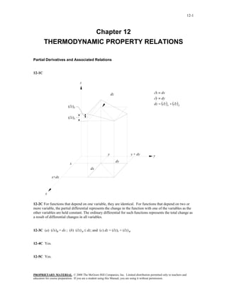
12-1C
z
dz ∂x ≡ dx
∂y ≡ dy
dz = (∂z ) x + (∂z ) y
(∂z)y
(∂z)x
y y + dy y
dy
x
dx
x+dx
x
12-2C For functions that depend on one variable, they are identical. For functions that depend on two or
more variable, the partial differential represents the change in the function with one of the variables as the
other variables are held constant. The ordinary differential for such functions represents the total change as
a result of differential changes in all variables.
12-3C (a) (∂x)y = dx ; (b) (∂z) y ≤ dz; and (c) dz = (∂z)x + (∂z) y
12-4C Yes.
12-5C Yes.
PROPRIETARY MATERIAL. © 2008 The McGraw-Hill Companies, Inc. Limited distribution permitted only to teachers and
educators for course preparation. If you are a student using this Manual, you are using it without permission.
- 2. 12-2
12-6 Air at a specified temperature and specific volume is considered. The changes in pressure
corresponding to a certain increase of different properties are to be determined.
Assumptions Air is an ideal gas.
Properties The gas constant of air is R = 0.287 kPa·m3/kg·K (Table A-1).
Analysis An ideal gas equation can be expressed as P = RT/v. Noting that R is a constant and P = P(T, v),
⎛ ∂P ⎞ ⎛ ∂P ⎞ R dT RT dv
dP = ⎜ ⎟ dT + ⎜ ⎟ dv = −
⎝ ∂T ⎠v ⎝ ∂v ⎠ T v v2
(a) The change in T can be expressed as dT ≅ ΔT = 400 × 0.01 = 4.0 K. At v = constant,
(0.287 kPa ⋅ m 3 /kg ⋅ K)(4.0 K)
(dP )v =
R dT
= = 1.276 kPa
v 0.90 m 3 /kg
(b) The change in v can be expressed as dv ≅ Δv = 0.90 × 0.01 = 0.009 m3/kg. At T = constant,
RT dv (0.287 kPa ⋅ m 3 /kg ⋅ K)(400K)(0.009 m 3 /kg)
(dP )T =− =− = −1.276 kPa
v2 (0.90 m 3 /kg) 2
(c) When both v and T increases by 1%, the change in P becomes
dP = (dP)v + (dP )T = 1.276 + (−1.276) = 0
Thus the changes in T and v balance each other.
12-7 Helium at a specified temperature and specific volume is considered. The changes in pressure
corresponding to a certain increase of different properties are to be determined.
Assumptions Helium is an ideal gas
Properties The gas constant of helium is R = 2.0769 kPa·m3/kg·K (Table A-1).
Analysis An ideal gas equation can be expressed as P = RT/v. Noting that R is a constant and P = P(T, v ),
⎛ ∂P ⎞ ⎛ ∂P ⎞ R dT RT dv
dP = ⎜ ⎟ dT + ⎜ ⎟ dv = −
⎝ ∂T ⎠v ⎝ ∂v ⎠ T v v2
(a) The change in T can be expressed as dT ≅ ΔT = 400 × 0.01 = 4.0 K. At v = constant,
(2.0769 kPa ⋅ m 3 /kg ⋅ K)(4.0 K)
(dP )v =
R dT
= = 9.231 kPa
v 0.90 m 3 /kg
(b) The change in v can be expressed as d v ≅ Δ v = 0.90 × 0.01 = 0.009 m3/kg. At T = constant,
RT dv (2.0769 kPa ⋅ m 3 /kg ⋅ K)(400 K)(0.009 m 3 )
(dP )T =− = = −9.231 kPa
v2 (0.90 m 3 /kg) 2
(c) When both v and T increases by 1%, the change in P becomes
dP = (dP) v + (dP ) T = 9.231 + (−9.231) = 0
Thus the changes in T and v balance each other.
PROPRIETARY MATERIAL. © 2008 The McGraw-Hill Companies, Inc. Limited distribution permitted only to teachers and
educators for course preparation. If you are a student using this Manual, you are using it without permission.
- 3. 12-3
12-8 It is to be proven for an ideal gas that the P = constant lines on a T- v diagram are straight lines and
that the high pressure lines are steeper than the low-pressure lines.
Analysis (a) For an ideal gas Pv = RT or T = Pv/R. Taking the partial derivative of T with respect to v
holding P constant yields
⎛ ∂T ⎞ P T
⎜ ⎟ =
⎝ ∂v ⎠ P R
which remains constant at P = constant. Thus the derivative P = const
(∂T/∂v)P, which represents the slope of the P = const. lines
on a T-v diagram, remains constant. That is, the P = const.
lines are straight lines on a T-v diagram.
(b) The slope of the P = const. lines on a T-v diagram is equal
to P/R, which is proportional to P. Therefore, the high
pressure lines are steeper than low pressure lines on the T-v v
diagram.
12-9 A relation is to be derived for the slope of the v = constant lines on a T-P diagram for a gas that obeys
the van der Waals equation of state.
Analysis The van der Waals equation of state can be expressed as
1⎛ ⎞
⎟(v − b )
a
T= ⎜P + 2
R⎝ v ⎠
Taking the derivative of T with respect to P holding v constant,
⎛ ∂T ⎞ 1 v −b
⎜ ⎟ = (1 + 0)(v − b ) =
⎝ ∂P ⎠v R R
which is the slope of the v = constant lines on a T-P diagram.
PROPRIETARY MATERIAL. © 2008 The McGraw-Hill Companies, Inc. Limited distribution permitted only to teachers and
educators for course preparation. If you are a student using this Manual, you are using it without permission.
- 4. 12-4
12-10 Nitrogen gas at a specified state is considered. The cp and cv of the nitrogen are to be determined
using Table A-18, and to be compared to the values listed in Table A-2b.
Analysis The cp and cv of ideal gases depends on temperature only, and are expressed as cp(T) = dh(T)/dT
and cv(T) = du(T)/dT. Approximating the differentials as differences about 400 K, the cp and cv values are
determined to be
⎛ dh(T ) ⎞ ⎛ Δh(T ) ⎞ cp
c p (400 K ) = ⎜ ⎟ ≅⎜ ⎟
⎝ dT ⎠ T = 400 K ⎝ ΔT ⎠ T ≅ 400 K h
h(410 K ) − h(390 K )
=
(410 − 390)K
(11,932 − 11,347)/28.0 kJ/kg
=
(410 − 390)K
= 1.045 kJ/kg ⋅ K
(Compare: Table A-2b at 400 K → cp = 1.044 kJ/kg·K) T
⎛ du (T ) ⎞ ⎛ Δu (T ) ⎞
cv (400K ) = ⎜ ⎟ ≅⎜ ⎟
⎝ dT ⎠ T = 400 K ⎝ ΔT ⎠ T ≅ 400 K
u (410 K ) − u (390 K )
=
(410 − 390)K
(8,523 − 8,104)/28.0 kJ/kg
= = 0.748 kJ/kg ⋅ K
(410 − 390)K
(Compare: Table A-2b at 400 K → cv = 0.747 kJ/kg·K)
PROPRIETARY MATERIAL. © 2008 The McGraw-Hill Companies, Inc. Limited distribution permitted only to teachers and
educators for course preparation. If you are a student using this Manual, you are using it without permission.
- 5. 12-5
12-11E Nitrogen gas at a specified state is considered. The cp and cv of the nitrogen are to be determined
using Table A-18E, and to be compared to the values listed in Table A-2Eb.
Analysis The cp and cv of ideal gases depends on temperature only, and are expressed as cp(T) = dh(T)/dT
and cv(T) = du(T)/dT. Approximating the differentials as differences about 600 R, the cp and cv values are
determined to be
⎛ dh(T ) ⎞ ⎛ Δh(T ) ⎞
c p (600 R ) = ⎜ ⎟ ≅⎜ ⎟
⎝ dT ⎠T = 600 R ⎝ ΔT ⎠T ≅ 600 R
h(620 R ) − h(580 R )
=
(620 − 580)R
(4,307.1 − 4,028.7)/28.0 Btu/lbm
= = 0.249 Btu/lbm ⋅ R
(620 − 580)R
(Compare: Table A-2Eb at 600 R → cp = 0.248 Btu/lbm·R )
⎛ du (T ) ⎞ ⎛ Δu (T ) ⎞
cv (600 R ) = ⎜ ⎟ ≅⎜ ⎟
⎝ dT ⎠T = 600 R ⎝ ΔT ⎠T ≅ 600 R
u (620 R ) − u (580 R )
=
(620 − 580)R
(3,075.9 − 2,876.9)/28.0 Btu/lbm
= = 0.178 Btu/lbm ⋅ R
(620 − 580) R
(Compare: Table A-2Eb at 600 R → cv = 0.178 Btu/lbm·R)
PROPRIETARY MATERIAL. © 2008 The McGraw-Hill Companies, Inc. Limited distribution permitted only to teachers and
educators for course preparation. If you are a student using this Manual, you are using it without permission.
- 6. 12-6
12-12 The state of an ideal gas is altered slightly. The change in the specific volume of the gas is to be
determined using differential relations and the ideal-gas relation at each state.
Assumptions The gas is air and air is an ideal gas.
Properties The gas constant of air is R = 0.287 kPa·m3/kg·K (Table A-1).
Analysis (a) The changes in T and P can be expressed as
dT ≅ ΔT = (404 − 400)K = 4 K
dP ≅ ΔP = (96 − 100)kPa = −4 kPa
The ideal gas relation Pv = RT can be expressed as v = RT/P. Note that R is a constant and v = v (T, P).
Applying the total differential relation and using average values for T and P,
⎛ ∂v ⎞ ⎛ ∂v ⎞ R dT RT dP
dv = ⎜ ⎟ dT + ⎜ ⎟ dP = −
⎝ ∂T ⎠ P ⎝ ∂P ⎠ T P P2
⎛ 4K (402 K)(−4 kPa) ⎞
= (0.287 kPa ⋅ m 3 /kg ⋅ K)⎜ − ⎟
⎜ 98 kPa (98 kPa) 2 ⎟
⎝ ⎠
= (0.0117 m 3 /kg) + (0.04805 m 3 /kg) = 0.0598 m 3 /kg
(b) Using the ideal gas relation at each state,
RT1 (0.287 kPa ⋅ m 3 /kg ⋅ K)(400 K)
v1 = = = 1.1480 m 3 /kg
P1 100 kPa
RT2 (0.287 kPa ⋅ m 3 /kg ⋅ K)(404 K)
v2 = = = 1.2078 m 3 /kg
P2 96 kPa
Thus,
Δv = v 2 − v1 = 1.2078 − 1.1480 = 0.0598 m3 /kg
The two results are identical.
PROPRIETARY MATERIAL. © 2008 The McGraw-Hill Companies, Inc. Limited distribution permitted only to teachers and
educators for course preparation. If you are a student using this Manual, you are using it without permission.
- 7. 12-7
12-13 Using the equation of state P(v-a) = RT, the cyclic relation, and the reciprocity relation at constant v
are to be verified.
Analysis (a) This equation of state involves three variables P, v, and T. Any two of these can be taken as
the independent variables, with the remaining one being the dependent variable. Replacing x, y, and z by
P, v, and T, the cyclic relation can be expressed as
⎛ ∂P ⎞ ⎛ ∂v ⎞ ⎛ ∂T ⎞
⎜ ⎟ ⎜ ⎟ ⎜ ⎟ = −1
⎝ ∂v ⎠T ⎝ ∂T ⎠ P ⎝ ∂P ⎠v
where
RT ⎛ ∂P ⎞ − RT P
P= ⎯⎯→ ⎜ ⎟ = =−
v −a ⎝ ∂v ⎠ T (v − a )2 v −a
RT ⎛ ∂v ⎞ R
v= +a ⎯ ⎯→ ⎜ ⎟ =
P ⎝ ∂T ⎠ P P
P (v − a) ⎛ ∂T ⎞ v −a
T= ⎯
⎯→ ⎜ ⎟ =
R ⎝ ∂P ⎠ v R
Substituting,
⎛ ∂P ⎞ ⎛ ∂v ⎞ ⎛ ∂T ⎞ ⎛ P ⎞⎛ R ⎞⎛ v − a ⎞
⎜ ⎟ ⎜ ⎟ ⎜ ⎟ = ⎜− ⎟⎜ ⎟⎜ ⎟ = −1
⎝ ∂v ⎠T ⎝ ∂T ⎠ P ⎝ ∂P ⎠v ⎝ v − a ⎠⎝ P ⎠⎝ R ⎠
which is the desired result.
(b) The reciprocity rule for this gas at v = constant can be expressed as
⎛ ∂P ⎞ 1
⎜ ⎟ =
⎝ ∂T ⎠v (∂T / ∂P)v
P (v − a) ⎛ ∂T ⎞ v −a
T= ⎯⎯→ ⎜ ⎟ =
R ⎝ ∂P ⎠v R
RT ⎛ ∂P ⎞ R
P= ⎯ ⎯→ ⎜ ⎟ =
v −a ⎝ ∂T ⎠v v − a
We observe that the first differential is the inverse of the second one. Thus the proof is complete.
PROPRIETARY MATERIAL. © 2008 The McGraw-Hill Companies, Inc. Limited distribution permitted only to teachers and
educators for course preparation. If you are a student using this Manual, you are using it without permission.
- 8. 12-8
The Maxwell Relations
12-14 The validity of the last Maxwell relation for refrigerant-134a at a specified state is to be verified.
Analysis We do not have exact analytical property relations for refrigerant-134a, and thus we need to
replace the differential quantities in the last Maxwell relation with the corresponding finite quantities.
Using property values from the tables about the specified state,
⎛ ∂s ⎞ ? ⎛ ∂v ⎞
⎜ ⎟ =− ⎜ ⎟
⎝ ∂P ⎠ T ⎝ ∂T ⎠ P
⎛ Δs ⎞ ?
⎛ Δv ⎞
⎜ ⎟ ≅−⎜ ⎟
⎝ ΔP ⎠ T =80°C ⎝ ΔT ⎠ P =1200 kPa
⎛ s1400 kPa − s1000 kPa ⎞ ? ⎛ v 100°C − v 60° C ⎞
⎜ ⎟ ≅ −⎜ ⎟
⎜ (1400 − 1000 )kPa ⎟ ⎜ (100 − 60 )°C ⎟
⎝ ⎠ T =80°C ⎝ ⎠ P =1200kPa
(1.0056 − 1.0458)kJ/kg ⋅ K ? (0.022442 − 0.018404)m 3 /kg
≅−
(1400 − 1000)kPa (100 − 60)°C
− 1.005 × 10 − 4 m 3 /kg ⋅ K ≅ −1.0095 × 10 − 4 m 3 /kg ⋅ K
since kJ ≡ kPa·m³, and K ≡ °C for temperature differences. Thus the last Maxwell relation is satisfied.
PROPRIETARY MATERIAL. © 2008 The McGraw-Hill Companies, Inc. Limited distribution permitted only to teachers and
educators for course preparation. If you are a student using this Manual, you are using it without permission.
- 9. 12-9
12-15 EES Problem 12-14 is reconsidered. The validity of the last Maxwell relation for refrigerant 134a at
the specified state is to be verified.
Analysis The problem is solved using EES, and the solution is given below.
"Input Data:"
T=80 [C]
P=1200 [kPa]
P_increment = 200 [kPa]
T_increment = 20 [C]
P[2]=P+P_increment
P[1]=P-P_increment
T[2]=T+T_increment
T[1]=T-T_increment
DELTAP = P[2]-P[1]
DELTAT = T[2]-T[1]
v[1]=volume(R134a,T=T[1],P=P)
v[2]=volume(R134a,T=T[2],P=P)
s[1]=entropy(R134a,T=T,P=P[1])
s[2]=entropy(R134a,T=T,P=P[2])
DELTAs=s[2] - s[1]
DELTAv=v[2] - v[1]
"The partial derivatives in the last Maxwell relation (Eq. 11-19) is associated with the Gibbs
function and are approximated by the ratio of ordinary differentials:"
LeftSide =DELTAs/DELTAP*Convert(kJ,m^3-kPa) "[m^3/kg-K]" "at T = Const."
RightSide=-DELTAv/DELTAT "[m^3/kg-K]" "at P = Const."
SOLUTION
DELTAP=400 [kPa] RightSide=-0.000101 [m^3/kg-K]
DELTAs=-0.04026 [kJ/kg-K] s[1]=1.046 [kJ/kg-K]
DELTAT=40 [C] s[2]=1.006 [kJ/kg-K]
DELTAv=0.004038 [m^3/kg] T=80 [C]
LeftSide=-0.0001007 [m^3/kg-K] T[1]=60 [C]
P=1200 [kPa] T[2]=100 [C]
P[1]=1000 [kPa] T_increment=20 [C]
P[2]=1400 [kPa] v[1]=0.0184 [m^3/kg]
P_increment=200 [kPa] v[2]=0.02244 [m^3/kg]
PROPRIETARY MATERIAL. © 2008 The McGraw-Hill Companies, Inc. Limited distribution permitted only to teachers and
educators for course preparation. If you are a student using this Manual, you are using it without permission.
- 10. 12-10
12-16E The validity of the last Maxwell relation for steam at a specified state is to be verified.
Analysis We do not have exact analytical property relations for steam, and thus we need to replace the
differential quantities in the last Maxwell relation with the corresponding finite quantities. Using property
values from the tables about the specified state,
⎛ ∂s ⎞ ? ⎛ ∂v ⎞
⎜ ⎟ =− ⎜ ⎟
⎝ ∂P ⎠ T ⎝ ∂T ⎠ P
⎛ Δs ⎞ ?
⎛ Δv ⎞
⎜ ⎟ ≅− ⎜ ⎟
⎝ ΔP ⎠ T =800°F ⎝ ΔT ⎠ P = 400psia
⎛ s 450 psia − s 350 psia ⎞ ? ⎛ v 900° F − v 700° F ⎞
⎜ ⎟ ≅ −⎜ ⎟
⎜ (450 − 350)psia ⎟ ⎜ (900 − 700 )°F ⎟
⎝ ⎠ T =800°F ⎝ ⎠ P = 400psia
(1.6706 − 1.7009)Btu/lbm ⋅ R ? (1.9777 − 1.6507)ft 3 /lbm
≅−
(450 − 350)psia (900 − 700)°F
− 1.639 × 10 −3 ft 3 /lbm ⋅ R ≅ −1.635 × 10 −3 ft 3 /lbm ⋅ R
since 1 Btu ≡ 5.4039 psia·ft3, and R ≡ °F for temperature differences. Thus the fourth Maxwell relation is
satisfied.
12-17 Using the Maxwell relations, a relation for (∂s/∂P)T for a gas whose equation of state is P(v-b) = RT
is to be obtained.
RT
Analysis This equation of state can be expressed as v = + b . Then,
P
⎛ ∂v ⎞ R
⎜ ⎟ =
⎝ ∂T ⎠ P P
From the fourth Maxwell relation,
⎛ ∂s ⎞ ⎛ ∂v ⎞ R
⎜ ⎟ = −⎜ ⎟ =−
⎝ ∂P ⎠ T ⎝ ∂T ⎠ P P
PROPRIETARY MATERIAL. © 2008 The McGraw-Hill Companies, Inc. Limited distribution permitted only to teachers and
educators for course preparation. If you are a student using this Manual, you are using it without permission.
- 11. 12-11
12-18 Using the Maxwell relations, a relation for (∂s/∂v)T for a gas whose equation of state is (P-a/v2)(v-b)
= RT is to be obtained.
RT a
Analysis This equation of state can be expressed as P = + 2 . Then,
v −b v
⎛ ∂P ⎞ R
⎜ ⎟ =
⎝ ∂T ⎠ v v − b
From the third Maxwell relation,
⎛ ∂s ⎞ ⎛ ∂P ⎞ R
⎜ ⎟ =⎜ ⎟ =
⎝ ∂v ⎠ T ⎝ ∂T ⎠ v v − b
12-19 Using the Maxwell relations and the ideal-gas equation of state, a relation for (∂s/∂v)T for an ideal
gas is to be obtained.
RT
Analysis The ideal gas equation of state can be expressed as P = . Then,
v
⎛ ∂P ⎞ R
⎜ ⎟ =
⎝ ∂T ⎠ v v
From the third Maxwell relation,
⎛ ∂s ⎞ ⎛ ∂P ⎞ R
⎜ ⎟ =⎜ ⎟ =
⎝ ∂v ⎠ T ⎝ ∂T ⎠ v v
PROPRIETARY MATERIAL. © 2008 The McGraw-Hill Companies, Inc. Limited distribution permitted only to teachers and
educators for course preparation. If you are a student using this Manual, you are using it without permission.
- 12. 12-12
⎛ ∂P ⎞ k ⎛ ∂P ⎞
12-20 It is to be proven that ⎜ ⎟ = ⎜ ⎟
⎝ ∂T ⎠ s k − 1 ⎝ ∂T ⎠ v
Analysis Using the definition of cv ,
⎛ ∂s ⎞ ⎛ ∂s ⎞ ⎛ ∂P ⎞
cv = T ⎜ ⎟ = T⎜ ⎟ ⎜ ⎟
⎝ ∂T ⎠ v ⎝ ∂P ⎠ v ⎝ ∂T ⎠ v
⎛ ∂s ⎞ ⎛ ∂v ⎞
Substituting the first Maxwell relation ⎜ ⎟ = −⎜ ⎟ ,
⎝ ∂P ⎠ v ⎝ ∂T ⎠ s
⎛ ∂v ⎞ ⎛ ∂P ⎞
cv = −T ⎜ ⎟ ⎜ ⎟
⎝ ∂T ⎠ s ⎝ ∂T ⎠ v
Using the definition of cp,
⎛ ∂s ⎞ ⎛ ∂s ⎞ ⎛ ∂v ⎞
c p = T⎜ ⎟ = T⎜ ⎟ ⎜ ⎟
⎝ ∂T ⎠ P ⎝ ∂v ⎠ P ⎝ ∂T ⎠ P
⎛ ∂s ⎞ ⎛ ∂P ⎞
Substituting the second Maxwell relation ⎜ ⎟ =⎜ ⎟ ,
⎝ ∂v ⎠ P ⎝ ∂T ⎠ s
⎛ ∂P ⎞ ⎛ ∂v ⎞
cp = T⎜ ⎟ ⎜ ⎟
⎝ ∂T ⎠ s ⎝ ∂T ⎠ P
From Eq. 12-46,
2
⎛ ∂v ⎞ ⎛ ∂P ⎞
c p − cv = −T ⎜ ⎟ ⎜ ⎟
⎝ ∂T ⎠ P ⎝ ∂v ⎠ T
Also,
k cp
=
k −1 c p − cv
Then,
⎛ ∂P ⎞ ⎛ ∂v ⎞
⎜ ⎟ ⎜ ⎟
k ⎝ ∂T ⎠ s ⎝ ∂T ⎠ P ⎛ ∂P ⎞ ⎛ ∂T ⎞ ⎛ ∂v ⎞
=− = −⎜ ⎟ ⎜ ⎟ ⎜ ⎟
k −1 2
⎛ ∂v ⎞ ⎛ ∂P ⎞ ⎝ ∂T ⎠ s ⎝ ∂v ⎠ P ⎝ ∂P ⎠ T
⎜ ⎟ ⎜ ⎟
⎝ ∂T ⎠ P ⎝ ∂v ⎠ T
Substituting this into the original equation in the problem statement produces
⎛ ∂P ⎞ ⎛ ∂P ⎞ ⎛ ∂T ⎞ ⎛ ∂v ⎞ ⎛ ∂P ⎞
⎜ ⎟ = −⎜ ⎟ ⎜ ⎟ ⎜ ⎟ ⎜ ⎟
⎝ ∂T ⎠ s ⎝ ∂T ⎠ s ⎝ ∂v ⎠ P ⎝ ∂P ⎠ T ⎝ ∂T ⎠ v
But, according to the cyclic relation, the last three terms are equal to −1. Then,
⎛ ∂P ⎞ ⎛ ∂P ⎞
⎜ ⎟ =⎜ ⎟
⎝ ∂T ⎠ s ⎝ ∂T ⎠ s
PROPRIETARY MATERIAL. © 2008 The McGraw-Hill Companies, Inc. Limited distribution permitted only to teachers and
educators for course preparation. If you are a student using this Manual, you are using it without permission.
- 13. 12-13
12-21 It is to be shown how T, v, u, a, and g could be evaluated from the thermodynamic function h = h(s,
P).
Analysis Forming the differential of the given expression for h produces
⎛ ∂h ⎞ ⎛ ∂h ⎞
dh = ⎜ ⎟ ds + ⎜ ⎟ dP
⎝ ∂s ⎠ P ⎝ ∂P ⎠ s
Solving the dh Gibbs equation gives
dh = Tds + vdP
Comparing the coefficient of these two expressions
⎛ ∂h ⎞
T =⎜ ⎟
⎝ ∂s ⎠ P
⎛ ∂h ⎞
v =⎜ ⎟
⎝ ∂P ⎠ s
both of which can be evaluated for a given P and s.
From the definition of the enthalpy,
⎛ ∂h ⎞
u = h − Pv = h-P⎜ ⎟
⎝ ∂P ⎠ s
Similarly, the definition of the Helmholtz function,
⎛ ∂h ⎞ ⎛ ∂h ⎞
a = u − Ts = h − P⎜ ⎟ − s⎜ ⎟
⎝ ∂P ⎠ s ⎝ ∂s ⎠ P
while the definition of the Gibbs function gives
⎛ ∂h ⎞
q = h − Ts = h − s⎜ ⎟
⎝ ∂s ⎠ P
All of these can be evaluated for a given P and s and the fundamental h(s,P) equation.
PROPRIETARY MATERIAL. © 2008 The McGraw-Hill Companies, Inc. Limited distribution permitted only to teachers and
educators for course preparation. If you are a student using this Manual, you are using it without permission.
- 14. 12-14
The Clapeyron Equation
12-22C It enables us to determine the enthalpy of vaporization from hfg at a given temperature from the P,
v, T data alone.
12-23C It is assumed that vfg ≅ vg ≅ RT/P, and hfg ≅ constant for small temperature intervals.
12-24 Using the Clapeyron equation, the enthalpy of vaporization of steam at a specified pressure is to be
estimated and to be compared to the tabulated data.
Analysis From the Clapeyron equation,
⎛ dP ⎞
h fg = Tv fg ⎜ ⎟
⎝ dT ⎠ sat
⎛ ΔP ⎞
≅ T (v g − v f ) @300 kPa ⎜ ⎟
⎝ ΔT ⎠ sat, 300 kPa
⎛ (325 − 275)kPa ⎞
= Tsat @300 kPa (v g − v f ) @300 kPa ⎜ ⎟
⎜ Tsat @325 kPa − Tsat @275 kPa ⎟
⎝ ⎠
3 ⎛ 50 kPa ⎞
= (133.52 + 273.15 K)(0.60582 − 0.001073 m /kg)⎜ ⎜ (136.27 − 130.58)°C ⎟
⎟
⎝ ⎠
= 2159.9 kJ/kg
The tabulated value of hfg at 300 kPa is 2163.5 kJ/kg.
PROPRIETARY MATERIAL. © 2008 The McGraw-Hill Companies, Inc. Limited distribution permitted only to teachers and
educators for course preparation. If you are a student using this Manual, you are using it without permission.
- 15. 12-15
12-25 The hfg and sfg of steam at a specified temperature are to be calculated using the Clapeyron equation
and to be compared to the tabulated data.
Analysis From the Clapeyron equation,
⎛ dP ⎞
h fg = Tv fg ⎜ ⎟
⎝ dT ⎠ sat
⎛ ΔP ⎞
≅ T (v g − v f ) @120°C ⎜ ⎟
⎝ ΔT ⎠ sat,120°C
⎛ Psat @125°C − Psat @115°C ⎞
= T (v g − v f ) @120°C ⎜
⎜
⎟
⎟
⎝ 125°C − 115°C ⎠
⎛ (232.23 − 169.18)kPa ⎞
= (120 + 273.15 K)(0.89133 − 0.001060 m 3 /kg)⎜
⎜ ⎟
⎟
⎝ 10 K ⎠
= 2206.8 kJ/kg
Also,
h fg 2206.8 kJ/kg
s fg = = = 5.6131 kJ/kg ⋅ K
T (120 + 273.15) K
The tabulated values at 120°C are hfg = 2202.1 kJ/kg and sfg = 5.6013 kJ/kg·K.
PROPRIETARY MATERIAL. © 2008 The McGraw-Hill Companies, Inc. Limited distribution permitted only to teachers and
educators for course preparation. If you are a student using this Manual, you are using it without permission.
- 16. 12-16
12-26E [Also solved by EES on enclosed CD] The hfg of refrigerant-134a at a specified temperature is to be
calculated using the Clapeyron equation and Clapeyron-Clausius equation and to be compared to the
tabulated data.
Analysis (a) From the Clapeyron equation,
⎛ dP ⎞
h fg = Tv fg ⎜ ⎟
⎝ dT ⎠ sat
⎛ ΔP ⎞
≅ T (v g − v f ) @ 50°F ⎜ ⎟
⎝ ΔT ⎠ sat, 50° F
⎛ Psat @ 60 ° F − Psat @ 40 °F ⎞
= T (v g − v f ) @ 50°F ⎜
⎜
⎟
⎟
⎝ 60°F − 40°F ⎠
⎛ (72.152 − 49.776) psia ⎞
= (50 + 459.67 R)(0.79136 − 0.01270 ft 3 /lbm)⎜
⎜ ⎟
⎟
⎝ 20 R ⎠
= 444.0 psia ⋅ ft 3 /lbm = 82.16 Btu/lbm (0.2% error)
since 1 Btu = 5.4039 psia·ft3.
(b) From the Clapeyron-Clausius equation,
⎛P ⎞ h fg ⎛ 1 1 ⎞
ln⎜ 2
⎜P ⎟ ≅
⎟ ⎜ − ⎟
⎜T T ⎟
⎝ 1 ⎠ sat R ⎝ 1 2 ⎠ sat
⎛ 72.152 psia ⎞ h fg ⎛ 1 1 ⎞
⎜ 49.776 psia ⎟ ≅ 0.01946 Btu/lbm ⋅ R ⎜ 40 + 459.67 R − 60 + 459.67 R ⎟
ln⎜ ⎟
⎝ ⎠ ⎝ ⎠
h fg = 93.80 Btu/lbm (14.4% error)
The tabulated value of hfg at 50°F is 82.00 Btu/lbm.
PROPRIETARY MATERIAL. © 2008 The McGraw-Hill Companies, Inc. Limited distribution permitted only to teachers and
educators for course preparation. If you are a student using this Manual, you are using it without permission.
- 17. 12-17
12-27 EES The enthalpy of vaporization of steam as a function of temperature using Clapeyron equation
and steam data in EES is to be plotted.
Analysis The enthalpy of vaporization is determined using Clapeyron equation from
ΔP
h fg ,Clapeyron = Tv fg
ΔT
At 100ºC, for an increment of 5ºC, we obtain
T1 = T − Tincrement = 100 − 5 = 95°C
T2 = T + Tincrement = 100 + 5 = 105°C
P1 = Psat @ 95°C = 84.61 kPa
P2 = Psat @ 105°C = 120.90 kPa
ΔT = T2 − T1 = 105 − 95 = 10°C
ΔP = P2 − P1 = 120.90 − 84.61 = 36.29 kPa
v f @ 100°C = 0.001043 m 3 /kg
v g @ 100°C = 1.6720 m 3 /kg
v fg = v g − v f = 1.6720 − 0.001043 = 1.6710 m 3 /kg
Substituting,
ΔP 36.29 kPa
h fg ,Clapeyron = Tv fg = (100 + 273.15 K)(1.6710 m 3 /kg) = 2262.8 kJ/kg
ΔT 10 K
The enthalpy of vaporization from steam table is
h fg @ 100°C = 2256.4 m 3 /kg
The percent error in using Clapeyron equation is
2262.8 − 2256.4
PercentError = × 100 = 0.28%
2256.4
We repeat the analysis over the temperature range 10 to 200ºC using EES. Below, the copy of EES
solution is provided:
"Input Data:"
"T=100" "[C]"
T_increment = 5"[C]"
T[2]=T+T_increment"[C]"
T[1]=T-T_increment"[C]"
P[1] = pressure(Steam_iapws,T=T[1],x=0)"[kPa]"
P[2] = pressure(Steam_iapws,T=T[2],x=0)"[kPa]"
DELTAP = P[2]-P[1]"[kPa]"
DELTAT = T[2]-T[1]"[C]"
v_f=volume(Steam_iapws,T=T,x=0)"[m^3/kg]"
v_g=volume(Steam_iapws,T=T,x=1)"[m^3/kg]"
h_f=enthalpy(Steam_iapws,T=T,x=0)"[kJ/kg]"
h_g=enthalpy(Steam_iapws,T=T,x=1)"[kJ/kg]"
h_fg=h_g - h_f"[kJ/kg-K]"
v_fg=v_g - v_f"[m^3/kg]"
PROPRIETARY MATERIAL. © 2008 The McGraw-Hill Companies, Inc. Limited distribution permitted only to teachers and
educators for course preparation. If you are a student using this Manual, you are using it without permission.
- 18. 12-18
"The Clapeyron equation (Eq. 11-22) provides a means to calculate the enthalpy of vaporization,
h_fg at a given temperature by determining the slope of the saturation curve on a P-T diagram
and the specific volume of the saturated liquid and satruated vapor at the temperature."
h_fg_Clapeyron=(T+273.15)*v_fg*DELTAP/DELTAT*Convert(m^3-kPa,kJ)"[kJ/kg]"
PercentError=ABS(h_fg_Clapeyron-h_fg)/h_fg*100"[%]"
hfg hfg,Clapeyron PercentError T
[kJ/kg] [kJ/kg] [%] [C]
2477.20 2508.09 1.247 10
2429.82 2451.09 0.8756 30
2381.95 2396.69 0.6188 50
2333.04 2343.47 0.4469 70
2282.51 2290.07 0.3311 90
2229.68 2235.25 0.25 110
2173.73 2177.86 0.1903 130
2113.77 2116.84 0.1454 150
2014.17 2016.15 0.09829 180
1899.67 1900.98 0.06915 210
1765.50 1766.38 0.05015 240
2600
2500 hfg calculated by Clapeyron equation
2400
hfg [kJ/kg]
2300
hfg calculated by EES
2200
2100
2000
1900
1800
1700
0 50 100 150 200 250
T [C]
PROPRIETARY MATERIAL. © 2008 The McGraw-Hill Companies, Inc. Limited distribution permitted only to teachers and
educators for course preparation. If you are a student using this Manual, you are using it without permission.
- 19. 12-19
12-28 A substance is heated in a piston-cylinder device until it turns from saturated liquid to saturated
vapor at a constant pressure and temperature. The boiling temperature of this substance at a different
pressure is to be estimated.
Analysis From the Clapeyron equation,
⎛ dP ⎞ h fg (5 kPa ⋅ m 3 )/(0.002 kg)
⎜ ⎟ = = = 14.16 kPa/K Weight
⎝ dT ⎠ sat Tv fg (353 K)(1× 10 −3 m 3 )/(0.002 kg)
Using the finite difference approximation,
⎛ dP ⎞ ⎛ P − P1 ⎞ 200 kPa
⎜ ⎟ ≈⎜ 2⎜ ⎟
⎟ 80°C Q
⎝ dT ⎠ sat ⎝ T2 − T1 ⎠ sat
2 grams
Solving for T2, Sat. liquid
P2 − P1 (180 − 200)kPa
T2 = T1 + = 353 K + = 351.6 K
dP / dT 14.16 kPa/K
12-29 A substance is heated in a piston-cylinder device until it turns from saturated liquid to saturated
vapor at a constant pressure and temperature. The saturation pressure of this substance at a different
temperature is to be estimated.
Analysis From the Clapeyron equation, Weight
3
⎛ dP ⎞ h fg (5 kPa ⋅ m )/(0.002 kg)
⎜ ⎟ = = = 14.16 kPa/K
⎝ dT ⎠ sat Tv fg (353 K)(1× 10 −3 m 3 )/(0.002 kg)
200 kPa
Using the finite difference approximation, 80°C Q
2 grams
⎛ dP ⎞ ⎛ P − P1 ⎞ Sat. liquid
⎜ ⎟ ≈⎜ 2 ⎟
⎝ dT ⎠ sat ⎜ T2 − T1 ⎟ sat
⎝ ⎠
Solving for P2,
dP
P2 = P1 + (T2 − T1 ) = 200 kPa + (14.16 kPa/K )(373 − 353)K = 483.2 kPa
dT
PROPRIETARY MATERIAL. © 2008 The McGraw-Hill Companies, Inc. Limited distribution permitted only to teachers and
educators for course preparation. If you are a student using this Manual, you are using it without permission.
- 20. 12-20
12-30 A substance is heated in a piston-cylinder device until it turns from saturated liquid to saturated
vapor at a constant pressure and temperature. The sfg of this substance at a different temperature is to be
estimated.
Analysis From the Clapeyron equation,
Weight
⎛ dP ⎞ h fg s fg
⎜ ⎟ = =
⎝ dT ⎠ sat Tv fg v fg
200 kPa
Solving for sfg,
80°C Q
h fg (5 kJ)/(0.002 kg) 2 grams
s fg = = = 7.082 kJ/kg ⋅ K Sat. liquid
T 353 K
Alternatively,
⎛ dP ⎞ 1× 10 -3 m 3
s fg = ⎜ ⎟ v fg = (14.16 kPa/K ) = 7.08 kPa ⋅ m 3 /kg ⋅ K = 7.08 kJ/kg ⋅ K
⎝ dT ⎠ sat 0.002 kg
⎛ ∂ (h fg / T ) ⎞
12-31 It is to be shown that c p , g − c p , f = T ⎜ ⎟ + v fg ⎛ ∂P ⎞ .
⎜ ⎟
⎜ ∂T ⎟ ⎝ ∂T ⎠ sat
⎝ ⎠P
Analysis The definition of specific heat and Clapeyron equation are
⎛ ∂h ⎞
cp = ⎜ ⎟
⎝ ∂T ⎠ P
⎛ dP ⎞ h fg
⎜ ⎟ =
⎝ dT ⎠ sat Tv fg
According to the definition of the enthalpy of vaporization,
h fg hg hf
= −
T T T
Differentiating this expression gives
⎛ ∂h fg / T ⎞ ⎛ ∂h / T ⎞ ⎛ ∂h / T ⎞
⎜ ⎟ =⎜ g ⎟ −⎜ f ⎟
⎜ ⎟ ⎜ ⎟ ⎜ ⎟
⎝ ∂T ⎠ P ⎝ ∂T ⎠ P ⎝ ∂T ⎠P
1 ⎛ ∂h g
⎞ ⎛ ∂h ⎞
⎟ − g −1⎜ f
h h
= ⎜ ⎟ + f
T ⎜ ∂T
⎟ 2 T ⎜ ∂T ⎟ 2
⎝⎠P T ⎝ ⎠P T
c p, g c p, f h g − h f
= − −
T T T2
Using Clasius-Clapeyron to replace the last term of this expression and solving for the specific heat
difference gives
⎛ ∂ (h fg / T ) ⎞
c p, g − c p, f = T ⎜ ⎟ + v fg ⎛ ∂P ⎞
⎜ ⎟
⎜ ∂T ⎟ ⎝ ∂T ⎠ sat
⎝ ⎠P
PROPRIETARY MATERIAL. © 2008 The McGraw-Hill Companies, Inc. Limited distribution permitted only to teachers and
educators for course preparation. If you are a student using this Manual, you are using it without permission.
- 21. 12-21
12-32E A table of properties for methyl chloride is given. The saturation pressure is to be estimated at two
different temperatures.
Analysis The Clapeyron equation is
⎛ dP ⎞ h fg
⎜ ⎟ =
⎝ dT ⎠ sat Tv fg
Using the finite difference approximation,
⎛ dP ⎞ ⎛ P2 − P1 ⎞ h fg
⎜ ⎟ ≈⎜ ⎟
⎜ T − T ⎟ = Tv
⎝ dT ⎠ sat ⎝ 2 1 ⎠ sat fg
Solving this for the second pressure gives for T2 = 110°F
h fg
P2 = P1 + (T2 − T1 )
Tv fg
154.85 Btu/lbm ⎛ 5.404 psia ⋅ ft 3 ⎞
= 116.7 psia + ⎜ ⎟(110 − 100)R
(560 R)(0.86332 ft 3 /lbm) ⎜
⎝ 1 Btu ⎟
⎠
= 134.0 psia
When T2 = 90°F
h fg
P2 = P1 + (T2 − T1 )
Tv fg
154.85 Btu/lbm ⎛ 5.404 psia ⋅ ft 3 ⎞
= 116.7 psia + ⎜ ⎟(90 − 100)R
(560 R)(0.86332 ft 3 /lbm) ⎜
⎝ 1 Btu ⎟
⎠
= 99.4 psia
PROPRIETARY MATERIAL. © 2008 The McGraw-Hill Companies, Inc. Limited distribution permitted only to teachers and
educators for course preparation. If you are a student using this Manual, you are using it without permission.
- 22. 12-22
12-33 Saturation properties for R-134a at a specified temperature are given. The saturation pressure is to be
estimated at two different temperatures.
Analysis From the Clapeyron equation,
⎛ dP ⎞ h fg 225.86 kPa ⋅ m 3 /kg
⎜ ⎟ = = = 2.692 kPa/K
⎝ dT ⎠ sat Tv fg (233 K)(0.36010 m 3 /kg)
Using the finite difference approximation,
⎛ dP ⎞ ⎛ P − P1 ⎞
⎜ ⎟ ≈⎜ 2⎜ ⎟
⎟
⎝ dT ⎠ sat ⎝ T2 − T1 ⎠ sat
Solving for P2 at −50°C
dP
P2 = P1 + (T2 − T1 ) = 51.25 kPa + (2.692 kPa/K )(223 − 233)K = 24.33 kPa
dT
Solving for P2 at −30°C
dP
P2 = P1 + (T2 − T1 ) = 51.25 kPa + (2.692 kPa/K )(243 − 233)K = 78.17 kPa
dT
PROPRIETARY MATERIAL. © 2008 The McGraw-Hill Companies, Inc. Limited distribution permitted only to teachers and
educators for course preparation. If you are a student using this Manual, you are using it without permission.
- 23. 12-23
General Relations for du, dh, ds, cv, and cp
12-34C Yes, through the relation
⎛ ∂c p ⎞ ⎛ 2 ⎞
⎜ ⎟ = −T ⎜ ∂ v ⎟
⎜ ∂P ⎟ ⎜ ∂T 2 ⎟
⎝ ⎠T ⎝ ⎠P
PROPRIETARY MATERIAL. © 2008 The McGraw-Hill Companies, Inc. Limited distribution permitted only to teachers and
educators for course preparation. If you are a student using this Manual, you are using it without permission.
- 24. 12-24
12-35 General expressions for Δu, Δh, and Δs for a gas whose equation of state is P(v-a) = RT for an
isothermal process are to be derived.
Analysis (a) A relation for Δu is obtained from the general relation
T2 v2 ⎛ ⎛ ∂P ⎞ ⎞
Δu = u 2 − u1 = ∫ T1
cv dT + ∫v 1
⎜T ⎜ ⎟
⎜ ⎝ ∂T ⎟ − P ⎟dv
⎝ ⎠v ⎠
The equation of state for the specified gas can be expressed as
RT ⎛ ∂P ⎞ R
P= ⎯⎯→ ⎜ ⎟ =
v −a ⎝ ∂T ⎠v v − a
Thus,
⎛ ∂P ⎞ RT
T⎜ ⎟ −P = −P = P−P = 0
⎝ ∂T ⎠v v −a
T2
Substituting, Δu = ∫T1
cv dT
(b) A relation for Δh is obtained from the general relation
⎛ ∂v ⎞ ⎞
⎜v − T ⎛
T2 P2
Δh = h2 − h1 = ∫ T1
c P dT + ∫ P1
⎜
⎝
⎜ ⎟ ⎟dP
⎝ ∂T ⎠ P ⎟
⎠
The equation of state for the specified gas can be expressed as
RT ⎛ ∂v ⎞ R
v= +a ⎯
⎯→ ⎜ ⎟ =
P ⎝ ∂T ⎠ P P
Thus,
⎛ ∂v ⎞ R
v −T⎜ ⎟ = v − T = v − (v − a ) = a
⎝ ∂T ⎠ P P
Substituting,
c p dT + a(P2 − P1 )
T2 P2 T2
Δh = ∫T1
c p dT + ∫ P1
a dP = ∫T1
(c) A relation for Δs is obtained from the general relation
T2 cp P2 ⎛ ∂v ⎞
Δs = s 2 − s1 = ∫
T1 T
dT − ∫P1
⎜ ⎟ dP
⎝ ∂T ⎠ P
Substituting (∂v/∂T)P = R/T,
T2 cp P2 ⎛R⎞ T2 cp P2
Δs = ∫
T1 T
dT − ∫P1
⎜ ⎟ dP =
⎝ P ⎠P ∫T1 T
dT − R ln
P1
For an isothermal process dT = 0 and these relations reduce to
P2
Δu = 0, Δh = a(P2 − P1 ), and Δs = − Rln
P1
PROPRIETARY MATERIAL. © 2008 The McGraw-Hill Companies, Inc. Limited distribution permitted only to teachers and
educators for course preparation. If you are a student using this Manual, you are using it without permission.
- 25. 12-25
12-36 General expressions for (∂u/∂P)T and (∂h/∂v)T in terms of P, v, and T only are to be derived.
Analysis The general relation for du is
⎛ ⎛ ∂P ⎞ ⎞
du = cv dT + ⎜ T ⎜ ⎟
⎜ ⎝ ∂T ⎟ − P ⎟dv
⎝ ⎠v ⎠
Differentiating each term in this equation with respect to P at T = constant yields
⎛ ∂u ⎞ ⎛ ⎛ ∂P ⎞ ⎞⎛ ∂v ⎞ ⎛ ∂P ⎞ ⎛ ∂v ⎞ ⎛ ∂v ⎞
⎜ ⎟ = 0 + ⎜T ⎜ ⎟
⎜ ⎝ ∂T ⎠ − P ⎟⎜ ∂P ⎟ = T ⎜ ∂T ⎟ ⎜ ∂P ⎟ − P⎜ ∂P ⎟
⎟
⎝ ∂P ⎠ T ⎝ v ⎠⎝ ⎠T ⎝ ⎠v ⎝ ⎠T ⎝ ⎠T
Using the properties P, T, v, the cyclic relation can be expressed as
⎛ ∂P ⎞ ⎛ ∂T ⎞ ⎛ ∂v ⎞ ⎛ ∂P ⎞ ⎛ ∂v ⎞ ⎛ ∂v ⎞
⎜ ⎟ ⎜ ⎟ ⎜ ⎟ = −1 ⎯
⎯→ ⎜ ⎟ ⎜ ⎟ = −⎜ ⎟
⎝ ∂T ⎠v ⎝ ∂v ⎠ P ⎝ ∂P ⎠ T ⎝ ∂T ⎠ v ⎝ ∂P ⎠ T ⎝ ∂T ⎠ P
Substituting, we get
⎛ ∂u ⎞ ⎛ ∂v ⎞ ⎛ ∂v ⎞
⎜ ⎟ = −T ⎜ ⎟ − P⎜ ⎟
⎝ ∂P ⎠ T ⎝ ∂T ⎠ P ⎝ ∂P ⎠ T
The general relation for dh is
⎛ ⎛ ∂v ⎞ ⎞
dh = c p dT + ⎜v − T ⎜
⎜ ⎟ ⎟dP
⎝ ⎝ ∂T ⎠ P ⎟
⎠
Differentiating each term in this equation with respect to v at T = constant yields
⎛ ∂h ⎞ ⎛ ⎛ ∂v ⎞ ⎞⎛ ∂P ⎞ ⎛ ∂P ⎞ ⎛ ∂v ⎞ ⎛ ∂P ⎞
⎜ ⎟ = 0 + ⎜v − T ⎜
⎜ ⎟ ⎟⎜⎟⎝ ∂v ⎟ = v ⎜ ∂v ⎟ − T ⎜ ∂T ⎟ ⎜ ∂v ⎟
⎝ ∂v ⎠ T ⎝ ⎝ ∂T ⎠ P ⎠ ⎠T ⎝ ⎠T ⎝ ⎠P ⎝ ⎠T
Using the properties v, T, P, the cyclic relation can be expressed as
⎛ ∂v ⎞ ⎛ ∂T ⎞ ⎛ ∂P ⎞ ⎛ ∂v ⎞ ⎛ ∂P ⎞ ⎛ ∂T ⎞
⎜ ⎟ ⎜ ⎟ ⎜ ⎟ = −1 ⎯
⎯→ ⎜ ⎟ ⎜ ⎟ = −⎜ ⎟
⎝ ∂T ⎠ P ⎝ ∂P ⎠ v ⎝ ∂v ⎠ T ⎝ ∂T ⎠ P ⎝ ∂v ⎠ T ⎝ ∂P ⎠ v
Substituting, we get
⎛ ∂h ⎞ ⎛ ∂P ⎞ ⎛ ∂T ⎞
⎜ ⎟ =v⎜ ⎟ +T⎜ ⎟
⎝ ∂v ⎠ T ⎝ ∂v ⎠ T ⎝ ∂P ⎠ v
PROPRIETARY MATERIAL. © 2008 The McGraw-Hill Companies, Inc. Limited distribution permitted only to teachers and
educators for course preparation. If you are a student using this Manual, you are using it without permission.
- 26. 12-26
12-37E The specific heat difference cp-cv for liquid water at 1000 psia and 150°F is to be estimated.
Analysis The specific heat difference cp - cv is given as
2
⎛ ∂v ⎞ ⎛ ∂P ⎞
c p − cv = −T ⎜ ⎟ ⎜ ⎟
⎝ ∂T ⎠ P ⎝ ∂v ⎠ T
Approximating differentials by differences about the specified state,
2
⎛ Δv ⎞ ⎛ ΔP ⎞
c p − cv ≅ −T ⎜ ⎟ ⎜ ⎟
⎝ ΔT ⎠ P =1000 psia ⎝ Δv ⎠ T =150°F
2
⎛ v 175° F − v 125° F ⎞ ⎛ (1500 − 500)psia ⎞
= −(150 + 459.67 R )⎜ ⎟ ⎜ ⎟
⎜ (175 − 125)°F ⎟ ⎜ ⎟
⎝ ⎠ P =1000psia ⎝ v 1500 psia − v 500 psia ⎠ T =150° F
2
⎛ (0.016427 − 0.016177)ft 3 /lbm ⎞ ⎛ 1000 psia ⎞
= −(609.67 R)⎜ ⎟ ⎜ ⎟
⎜ 50 R ⎟ ⎜ (0.016267 − 0.016317)ft 3 /lbm ⎟
⎝ ⎠ ⎝ ⎠
= 0.3081 psia ⋅ ft 3 /lbm ⋅ R
= 0.0570 Btu/lbm ⋅ R (1 Btu = 5.4039 psia ⋅ ft 3 )
12-38 The volume expansivity β and the isothermal compressibility α of refrigerant-134a at 200 kPa and
30°C are to be estimated.
Analysis The volume expansivity and isothermal compressibility are expressed as
1 ⎛ ∂v ⎞ 1 ⎛ ∂v ⎞
β= ⎜ ⎟ and α = − ⎜ ⎟
v ⎝ ∂T ⎠ P v ⎝ ∂P ⎠ T
Approximating differentials by differences about the specified state,
1 ⎛ Δv ⎞ 1 ⎛ v 40°C − v 20°C ⎞
β≅ ⎜ ⎟ = ⎜ ⎟
v ⎝ ΔT ⎠ P = 200kPa v ⎜ (40 − 20)°C
⎝
⎟
⎠ P = 200 kPa
1 ⎛ (0.12322 − 0.11418) m 3 /kg ⎞
= ⎜ ⎟
0.11874 m 3 /kg ⎜
⎝ 20 K ⎟
⎠
= 0.00381 K −1
and
1 ⎛ Δv ⎞ 1 ⎛ v 240 kPa − v 180 kPa ⎞
α ≅− ⎜ ⎟ =− ⎜ ⎟
v ⎝ ΔP ⎠ T =30°C v ⎜ (240 − 180)kPa
⎝
⎟
⎠ T =30°C
1 ⎛ (0.09812 − 0.13248)m 3 /kg ⎞
=− ⎜ ⎟
0.11874 m /kg ⎜
3
⎝ 60 kPa ⎟
⎠
= 0.00482 kPa −1
PROPRIETARY MATERIAL. © 2008 The McGraw-Hill Companies, Inc. Limited distribution permitted only to teachers and
educators for course preparation. If you are a student using this Manual, you are using it without permission.
- 27. 12-27
⎛ ∂P ⎞ ⎛ ∂v ⎞
12-39 It is to be shown that c p − cv = T ⎜ ⎟ ⎜ ⎟ .
⎝ ∂T ⎠ v ⎝ ∂T ⎠ P
Analysis We begin by taking the entropy to be a function of specific volume and temperature. The
differential of the entropy is then
⎛ ∂s ⎞ ⎛ ∂s ⎞
ds = ⎜ ⎟ dT + ⎜ ⎟ dv
⎝ ∂T ⎠ v ⎝ ∂v ⎠ T
⎛ ∂s ⎞ c
Substituting ⎜ ⎟ = v from Eq. 12-28 and the third Maxwell equation changes this to
⎝ ∂T ⎠ v T
cv ⎛ ∂P ⎞
ds = dT + ⎜ ⎟ dv
T ⎝ ∂T ⎠v
Taking the entropy to be a function of pressure and temperature,
⎛ ∂s ⎞ ⎛ ∂s ⎞
ds = ⎜ ⎟ dT + ⎜ ⎟ dP
⎝ ∂T ⎠ P ⎝ ∂P ⎠ T
⎛ ∂s ⎞ cp
Combining this result with ⎜ ⎟ = from Eq. 12-34 and the fourth Maxwell equation produces
⎝ ∂T ⎠ P T
cp ⎛ ∂v ⎞
ds = dT − ⎜ ⎟ dP
T ⎝ ∂T ⎠ P
Equating the two previous ds expressions and solving the result for the specific heat difference,
⎛ ∂v ⎞ ⎛ ∂P ⎞
(c p − cv )dT = T ⎜ ⎟ dP + ⎜ ⎟ dv
⎝ ∂T ⎠ P ⎝ ∂T ⎠ v
Taking the pressure to be a function of temperature and volume,
⎛ ∂P ⎞ ⎛ ∂P ⎞
dP = ⎜ ⎟ dT + ⎜ ⎟ dv
⎝ ∂T ⎠ v ⎝ ∂v ⎠ T
When this is substituted into the previous expression, the result is
⎛ ∂v ⎞ ⎛ ∂P ⎞ ⎡⎛ ∂v ⎞ ⎛ ∂P ⎞ ⎛ ∂P ⎞ ⎤
(c p − cv )dT = T ⎜ ⎟ ⎜ ⎟ dT + T ⎢⎜ ⎟ ⎜ ⎟ ⎜ ⎟ ⎥ dv
⎝ ∂T ⎠ P ⎝ ∂T ⎠ v ⎣⎝ ∂T ⎠ P ⎝ ∂v ⎠ T ⎝ ∂T ⎠ v ⎦
According to the cyclic relation, the term in the bracket is zero. Then, canceling the common dT term,
⎛ ∂P ⎞ ⎛ ∂v ⎞
c p − cv = T ⎜ ⎟ ⎜ ⎟
⎝ ∂T ⎠ v ⎝ ∂T ⎠ P
PROPRIETARY MATERIAL. © 2008 The McGraw-Hill Companies, Inc. Limited distribution permitted only to teachers and
educators for course preparation. If you are a student using this Manual, you are using it without permission.
- 28. 12-28
12-40 It is to be proven that the definition for temperature T = (∂u / ∂s ) v reduces the net entropy change of
two constant-volume systems filled with simple compressible substances to zero as the two systems
approach thermal equilibrium.
Analysis The two constant-volume systems form an isolated system shown here
For the isolated system
dS tot = dS A + dS B ≥ 0
Assume S = S (u , v ) VA =const. Isolated
TA system
Then, boundary
⎛ ∂s ⎞ ⎛ ∂s ⎞
ds = ⎜ ⎟ du + ⎜ ⎟ dv VB =const.
⎝ ∂u ⎠ v ⎝ ∂v ⎠ u TB
Since v = const. and dv = 0 ,
⎛ ∂s ⎞
ds = ⎜ ⎟ du
⎝ ∂u ⎠ v
and from the definition of temperature from the problem statement,
du du
=
(∂u / ∂s ) v T
Then,
du A du B
dS tot = m A + mB
TA TB
The first law applied to the isolated system yields
E in − E out = dU
0 = dU ⎯
⎯→ m A du A + m B du B = 0 ⎯
⎯→ m B du B = −m A du A
Now, the entropy change may be expressed as
⎛ 1 1 ⎞ ⎛ T − TA ⎞
dS tot = m A du A ⎜
⎜T − T ⎟ = m A du A ⎜ B
⎟ ⎜ T T ⎟
⎟
⎝ A B ⎠ ⎝ A B ⎠
As the two systems approach thermal equilibrium,
lim dS tot = 0
T A → TB
PROPRIETARY MATERIAL. © 2008 The McGraw-Hill Companies, Inc. Limited distribution permitted only to teachers and
educators for course preparation. If you are a student using this Manual, you are using it without permission.
- 29. 12-29
12-41 The internal energy change of air between two specified states is to be compared for two equations
of states.
Assumptions Constant specific heats for air can be used.
Properties For air at the average temperature (20+300)/2=160°C=433 K, cv = 0.731 kJ/kg⋅K (Table A-2b).
Analysis Solving the equation of state for P gives
RT
P=
v −a
Then,
⎛ ∂P ⎞ R
⎜ ⎟ =
⎝ ∂T ⎠v v − a
Using equation 12-29,
⎡ ⎛ ∂P ⎞ ⎤
du = cv dT + ⎢T ⎜ ⎟ − P ⎥ dv
⎣ ⎝ ∂T ⎠v ⎦
Substituting,
⎛ RT RT ⎞
du = cv dT + ⎜ − ⎟dv
⎝ v −a v −a⎠
= cv dT
Integrating this result between the two states with constant specific heats gives
u 2 − u1 = cv (T2 − T1 ) = (0.731 kJ/kg ⋅ K)(300 − 20)K = 205 kJ/kg
The ideal gas model for the air gives
du = cv dT
which gives the same answer.
PROPRIETARY MATERIAL. © 2008 The McGraw-Hill Companies, Inc. Limited distribution permitted only to teachers and
educators for course preparation. If you are a student using this Manual, you are using it without permission.
- 30. 12-30
12-42 The enthalpy change of air between two specified states is to be compared for two equations of
states.
Assumptions Constant specific heats for air can be used.
Properties For air at the average temperature (20+300)/2=160°C=433 K, cp = 1.018 kJ/kg⋅K (Table A-2b).
Analysis Solving the equation of state for v gives
RT
v= +a
P
Then,
⎛ ∂v ⎞ R
⎜ ⎟ =
⎝ ∂T ⎠ P P
Using equation 12-35,
⎡ ⎛ ∂v ⎞ ⎤
dh = c p dT + ⎢v − T ⎜ ⎟ ⎥ dP
⎣ ⎝ ∂T ⎠ P ⎦
Substituting,
⎛ RT RT ⎞
dh = c p dT + ⎜ +a− ⎟dP
⎝ P P ⎠
= c p dT + adP
Integrating this result between the two states with constant specific heats gives
h2 − h1 = c p (T2 − T1 ) + a ( P2 − P1 )
= (1.018 kJ/kg ⋅ K)(300 − 20)K + (0.10 m 3 /kg)(600 − 100)kPa
= 335.0 kJ/kg
For an ideal gas,
dh = c p dT
which when integrated gives
h2 − h1 = c p (T2 − T1 ) = (1.018 kJ/kg ⋅ K)(300 − 20)K = 285.0 kJ/kg
PROPRIETARY MATERIAL. © 2008 The McGraw-Hill Companies, Inc. Limited distribution permitted only to teachers and
educators for course preparation. If you are a student using this Manual, you are using it without permission.
- 31. 12-31
12-43 The entropy change of air between two specified states is to be compared for two equations of states.
Assumptions Constant specific heats for air can be used.
Properties For air at the average temperature (20+300)/2=160°C=433 K, cp = 1.018 kJ/kg⋅K (Table A-2b)
and R = 0.287 kJ/kg⋅K (Table A-1).
Analysis Solving the equation of state for v gives
RT
v= +a
P
Then,
⎛ ∂v ⎞ R
⎜ ⎟ =
⎝ ∂T ⎠ P P
The entropy differential is
dT ⎛ ∂v ⎞
ds = c p −⎜ ⎟ dP
T ⎝ ∂T ⎠ P
dT dP
= cp −R
T P
which is the same as that of an ideal gas. Integrating this result between the two states with constant
specific heats gives
T2 P
s 2 − s1 = c p ln − R ln 2
T1 P1
573 K 600 kPa
= (1.018 kJ/kg ⋅ K)ln − (0.287 kJ/kg ⋅ K)ln
293 K 100 kPa
= 0.1686 kJ/kg ⋅ K
PROPRIETARY MATERIAL. © 2008 The McGraw-Hill Companies, Inc. Limited distribution permitted only to teachers and
educators for course preparation. If you are a student using this Manual, you are using it without permission.
- 32. 12-32
12-44 The internal energy change of helium between two specified states is to be compared for two
equations of states.
Properties For helium, cv = 3.1156 kJ/kg⋅K (Table A-2a).
Analysis Solving the equation of state for P gives
RT
P=
v −a
Then,
⎛ ∂P ⎞ R
⎜ ⎟ =
⎝ ∂T ⎠v v − a
Using equation 12-29,
⎡ ⎛ ∂P ⎞ ⎤
du = cv dT + ⎢T ⎜ ⎟ − P ⎥ dv
⎣ ⎝ ∂T ⎠v ⎦
Substituting,
⎛ RT RT ⎞
du = cv dT + ⎜ − ⎟dv
⎝v − a v − a ⎠
= cv dT
Integrating this result between the two states gives
u 2 − u1 = cv (T2 − T1 ) = (3.1156 kJ/kg ⋅ K)(300 − 20)K = 872.4 kJ/kg
The ideal gas model for the helium gives
du = cv dT
which gives the same answer.
PROPRIETARY MATERIAL. © 2008 The McGraw-Hill Companies, Inc. Limited distribution permitted only to teachers and
educators for course preparation. If you are a student using this Manual, you are using it without permission.
- 33. 12-33
12-45 The enthalpy change of helium between two specified states is to be compared for two equations of
states.
Properties For helium, cp = 5.1926 kJ/kg⋅K (Table A-2a).
Analysis Solving the equation of state for v gives
RT
v= +a
P
Then,
⎛ ∂v ⎞ R
⎜ ⎟ =
⎝ ∂T ⎠ P P
Using equation 12-35,
⎡ ⎛ ∂v ⎞ ⎤
dh = c p dT + ⎢v − T ⎜ ⎟ ⎥ dP
⎣ ⎝ ∂T ⎠ P ⎦
Substituting,
⎛ RT RT ⎞
dh = c p dT + ⎜ +a− ⎟dP
⎝ P P ⎠
= c p dT + adP
Integrating this result between the two states gives
h2 − h1 = c p (T2 − T1 ) + a ( P2 − P1 )
= (5.1926 kJ/kg ⋅ K)(300 − 20)K + (0.10 m 3 /kg)(600 − 100)kPa
= 1504 kJ/kg
For an ideal gas,
dh = c p dT
which when integrated gives
h2 − h1 = c p (T2 − T1 ) = (5.1926 kJ/kg ⋅ K)(300 − 20)K = 1454 kJ/kg
PROPRIETARY MATERIAL. © 2008 The McGraw-Hill Companies, Inc. Limited distribution permitted only to teachers and
educators for course preparation. If you are a student using this Manual, you are using it without permission.
- 34. 12-34
12-46 The entropy change of helium between two specified states is to be compared for two equations of
states.
Properties For helium, cp = 5.1926 kJ/kg⋅K and R = 2.0769 kJ/kg⋅K (Table A-2a).
Analysis Solving the equation of state for v gives
RT
v= +a
P
Then,
⎛ ∂v ⎞ R
⎜ ⎟ =
⎝ ∂T ⎠ P P
The entropy differential is
dT ⎛ ∂v ⎞
ds = c p −⎜ ⎟ dP
T ⎝ ∂T ⎠ P
dT dP
= cp −R
T P
which is the same as that of an ideal gas. Integrating this result between the two states gives
T2 P
s 2 − s1 = c p ln − R ln 2
T1 P1
573 K 600 kPa
= (5.1926 kJ/kg ⋅ K)ln − (2.0769 kJ/kg ⋅ K)ln
293 K 100 kPa
= −0.2386 kJ/kg ⋅ K
12-47 An expression for the volume expansivity of a substance whose equation of state is P (v − a) = RT
is to be derived.
Analysis Solving the equation of state for v gives
RT
v= +a
P
The specific volume derivative is then
⎛ ∂v ⎞ R
⎜ ⎟ =
⎝ ∂T ⎠ P P
The definition for volume expansivity is
1 ⎛ ∂v ⎞
β= ⎜ ⎟
v ⎝ ∂T ⎠ P
Combining these two equations gives
R
β=
RT + aP
PROPRIETARY MATERIAL. © 2008 The McGraw-Hill Companies, Inc. Limited distribution permitted only to teachers and
educators for course preparation. If you are a student using this Manual, you are using it without permission.
- 35. 12-35
v ⎛ T T T ⎞
12-48 The Helmholtz function of a substance has the form a = − RT ln − cT0 ⎜1 − ⎟
⎜ T + T ln T ⎟ . It is to
v0 ⎝ 0 0 0 ⎠
be shown how to obtain P, h, s, cv, and cp from this expression.
Analysis Taking the Helmholtz function to be a function of temperature and specific volume yields
⎛ ∂a ⎞ ⎛ ∂a ⎞
da = ⎜ ⎟ dT + ⎜ ⎟ dv
⎝ ∂T ⎠ v ⎝ ∂v ⎠ T
while the applicable Helmholtz equation is
da = − Pdv − sdT
Equating the coefficients of the two results produces
⎛ ∂a ⎞
P = −⎜ ⎟
⎝ ∂v ⎠ T
⎛ ∂a ⎞
s = −⎜ ⎟
⎝ ∂T ⎠ v
Taking the indicated partial derivatives of the Helmholtz function given in the problem statement reduces
these expressions to
RT
P=
v
v T
s = R ln + c ln
v0 T0
The definition of the enthalpy (h = u + Pv) and Helmholtz function (a = u−Ts) may be combined to give
h = u + Pv
= a + Ts + Pv
⎛ ∂a ⎞ ⎛ ∂a ⎞
= a −T⎜ ⎟ −v ⎜ ⎟
⎝ ∂T ⎠ v ⎝ ∂v ⎠ T
v ⎛ T T T ⎞ v T
= − RT ln − cT0 ⎜1 − ⎟
⎜ T + T ln T ⎟ + RT ln v − cT ln T + RT
v0 ⎝ 0 0 0 ⎠ 0 0
= cT0 + cT + RT
⎛ ∂s ⎞ c
According to ⎜ ⎟ = v given in the text (Eq. 12-28),
⎝ ∂T ⎠ v T
⎛ ∂s ⎞ c
cv = T ⎜ ⎟ =T =c
⎝ ∂T ⎠ v T
The preceding expression for the temperature indicates that the equation of state for the substance is the
same as that of an ideal gas. Then,
c p = R + cv = R + c
PROPRIETARY MATERIAL. © 2008 The McGraw-Hill Companies, Inc. Limited distribution permitted only to teachers and
educators for course preparation. If you are a student using this Manual, you are using it without permission.
- 36. 12-36
12-49 An expression for the volume expansivity of a substance whose equation of state
RT a
is P = − is to be derived.
v − b v (v + b)T 1 / 2
Analysis The definition for volume expansivity is
1 ⎛ ∂v ⎞
β= ⎜ ⎟
v ⎝ ∂T ⎠ P
According to the cyclic relation,
⎛ ∂v ⎞ ⎛ ∂P ⎞ ⎛ ∂T ⎞
⎜ ⎟ ⎜ ⎟ ⎜ ⎟ = −1
⎝ ∂T ⎠ P ⎝ ∂v ⎠ T ⎝ ∂P ⎠ v
which on rearrangement becomes
⎛ ∂P ⎞
⎜ ⎟
⎛ ∂v ⎞ ⎝ ∂T ⎠ v
⎜ ⎟ =−
⎝ ∂T ⎠ P ⎛ ∂P ⎞
⎜ ⎟
⎝ ∂v ⎠ T
Proceeding to perform the differentiations gives
⎛ ∂P ⎞ R a
⎜ ⎟ = +
⎝ ∂T ⎠ v v − b 2v (v + b)T 3 / 2
and
⎛ ∂P ⎞ RT a ⎡ 1 1 ⎤
⎜ ⎟ =− + 1/ 2 ⎢ 2 − 2 ⎥
⎝ ∂v ⎠ T (v − b) 2
bT ⎢v
⎣ (v + b) ⎥⎦
RT a 2v + b
=− +
(v − b) 2 T 1 / 2 v 2 (v + b) 2
Substituting these results into the definition of the volume expansivity produces
R a
+
1 v − b 2v (v + b)T 3 / 2
β=−
v − RT a 2v + b
2
+ 1/ 2 2
(v − b) T v (v + b) 2
PROPRIETARY MATERIAL. © 2008 The McGraw-Hill Companies, Inc. Limited distribution permitted only to teachers and
educators for course preparation. If you are a student using this Manual, you are using it without permission.
- 37. 12-37
12-50 An expression for the specific heat difference of a substance whose equation of state
RT a
is P = − is to be derived.
v − b v (v + b)T 1 / 2
Analysis The specific heat difference is expressed by
2
⎛ ∂v ⎞ ⎛ ∂P ⎞
c p − cv = −T ⎜ ⎟ ⎜ ⎟
⎝ ∂T ⎠ P ⎝ ∂v ⎠ T
According to the cyclic relation,
⎛ ∂v ⎞ ⎛ ∂P ⎞ ⎛ ∂T ⎞
⎜ ⎟ ⎜ ⎟ ⎜ ⎟ = −1
⎝ ∂T ⎠ P ⎝ ∂v ⎠ T ⎝ ∂P ⎠ v
which on rearrangement becomes
−1
⎛ ∂v ⎞ ⎛ ∂P ⎞ ⎛ ∂P ⎞
⎜ ⎟ = −⎜ ⎟ ⎜ ⎟
⎝ ∂T ⎠ P ⎝ ∂T ⎠ v ⎝ ∂v ⎠ T
Substituting this result into the expression for the specific heat difference gives
2 −1
⎛ ∂P ⎞ ⎛ ∂P ⎞
c p − cv = −T ⎜ ⎟ ⎜ ⎟
⎝ ∂T ⎠ v ⎝ ∂v ⎠ T
The appropriate partial derivatives of the equation of state are
⎛ ∂P ⎞ R a/2
⎜ ⎟ = +
⎝ ∂T ⎠v v − b v (v + b)T 3 / 2
⎛ ∂P ⎞ RT a ⎡ 1 1 ⎤
⎜ ⎟ =− + 1/ 2 ⎢ 2 − 2⎥
⎝ ∂v ⎠ T (v − b) 2
bT ⎢v
⎣ (v + b) ⎥
⎦
RT a 2v + b
=− 2
+ 1/ 2
(v − b) T v (v + b) 2
2
The difference in the specific heats is then
2
⎡ R a/2 ⎤
−T ⎢ + 3/ 2 ⎥
⎢ v − b v (v + b)T
⎣ ⎥
⎦
c p − cv =
RT a 2v + b
− +
(v − b) 2 T 1 / 2 v 2 (v + b) 2
PROPRIETARY MATERIAL. © 2008 The McGraw-Hill Companies, Inc. Limited distribution permitted only to teachers and
educators for course preparation. If you are a student using this Manual, you are using it without permission.
- 38. 12-38
RT a
12-51 An expression for the volume expansivity of a substance whose equation of state is P = −
v − b v 2T
is to be derived.
Analysis The definition for volume expansivity is
1 ⎛ ∂v ⎞
β= ⎜ ⎟
v ⎝ ∂T ⎠ P
According to the cyclic relation,
⎛ ∂v ⎞ ⎛ ∂P ⎞ ⎛ ∂T ⎞
⎜ ⎟ ⎜ ⎟ ⎜ ⎟ = −1
⎝ ∂T ⎠ P ⎝ ∂v ⎠ T ⎝ ∂P ⎠ v
which on rearrangement becomes
⎛ ∂P ⎞
⎜ ⎟
⎛ ∂v ⎞ ⎝ ∂T ⎠ v
⎜ ⎟ =−
⎝ ∂T ⎠ P ⎛ ∂P ⎞
⎜ ⎟
⎝ ∂v ⎠ T
Proceeding to perform the differentiations gives
⎛ ∂P ⎞ R a
⎜ ⎟ = +
⎝ ∂T ⎠ v v − b v 2 T 2
and
⎛ ∂P ⎞ RT 2a
⎜ ⎟ =− + 3
⎝ ∂v ⎠ T (v − b) 2
v T
Substituting these results into the definition of the volume expansivity produces
R a
+
1 v − b v 2T 2
β=−
v − RT 2a
2
+ 3
(v − b) v T
PROPRIETARY MATERIAL. © 2008 The McGraw-Hill Companies, Inc. Limited distribution permitted only to teachers and
educators for course preparation. If you are a student using this Manual, you are using it without permission.
- 39. 12-39
12-52 An expression for the isothermal compressibility of a substance whose equation of state
RT a
is P = − is to be derived.
v − b v 2T
Analysis The definition for the isothermal compressibility is
1 ⎛ ∂v ⎞
α=− ⎜ ⎟
v ⎝ ∂P ⎠ T
Now,
⎛ ∂P ⎞ − RT 2a
⎜ ⎟ = + 3
⎝ ∂v ⎠ T (v − b) 2
v T
Using the partial derivative properties,
1 1
α=− =−
⎛ ∂P ⎞ − RTv 2a
v⎜ ⎟ 2
+
⎝ ∂v ⎠ T (v − b) v 2T
⎛ ∂P ⎞
12-53 It is to be shown that β = α ⎜ ⎟ .
⎝ ∂T ⎠ v
Analysis The definition for the volume expansivity is
1 ⎛ ∂v ⎞
β= ⎜ ⎟
v ⎝ ∂T ⎠ P
The definition for the isothermal compressibility is
1 ⎛ ∂v ⎞
α=− ⎜ ⎟
v ⎝ ∂P ⎠ T
According to the cyclic relation,
⎛ ∂v ⎞ ⎛ ∂P ⎞ ⎛ ∂T ⎞
⎜ ⎟ ⎜ ⎟ ⎜ ⎟ = −1
⎝ ∂T ⎠ P ⎝ ∂v ⎠ T ⎝ ∂P ⎠ v
which on rearrangement becomes
⎛ ∂v ⎞ ⎛ ∂v ⎞ ⎛ ∂P ⎞
⎜ ⎟ = −⎜ ⎟ ⎜ ⎟
⎝ ∂T ⎠ P ⎝ ∂P ⎠ T ⎝ ∂T ⎠ v
When this is substituted into the definition of the volume expansivity, the result is
1 ⎛ ∂v ⎞ ⎛ ∂P ⎞
β=− ⎜ ⎟ ⎜ ⎟
v ⎝ ∂P ⎠ T ⎝ ∂T ⎠v
⎛ ∂P ⎞
= − α⎜ ⎟
⎝ ∂T ⎠ v
PROPRIETARY MATERIAL. © 2008 The McGraw-Hill Companies, Inc. Limited distribution permitted only to teachers and
educators for course preparation. If you are a student using this Manual, you are using it without permission.
- 40. 12-40
cp vα
12-54 It is to be demonstrated that k = =− .
cv (∂v / ∂P )s
Analysis The relations for entropy differential are
dT ⎛ ∂P ⎞
ds = cv +⎜ ⎟ dv
T ⎝ ∂T ⎠ v
dT ⎛ ∂v ⎞
ds = c p −⎜ ⎟ dP
T ⎝ ∂T ⎠ P
For fixed s, these basic equations reduce to
dT ⎛ ∂P ⎞
cv = −⎜ ⎟ dv
T ⎝ ∂T ⎠ v
dT ⎛ ∂v ⎞
cp =⎜ ⎟ dP
T ⎝ ∂T ⎠ P
Also, when s is fixed,
∂v ⎛ ∂v ⎞
=⎜ ⎟
∂P ⎝ ∂P ⎠ s
Forming the specific heat ratio from these expressions gives
⎛ ∂v ⎞ ⎛ ∂T ⎞
⎜ ⎟ ⎜ ⎟
⎝ ∂T ⎠ P ⎝ ∂P ⎠ v
k=−
⎛ ∂v ⎞
⎜ ⎟
⎝ ∂P ⎠ s
The cyclic relation is
⎛ ∂v ⎞ ⎛ ∂P ⎞ ⎛ ∂T ⎞
⎜ ⎟ ⎜ ⎟ ⎜ ⎟ = −1
⎝ ∂T ⎠ P ⎝ ∂v ⎠ T ⎝ ∂P ⎠ v
Solving this for the numerator of the specific heat ratio expression and substituting the result into this
numerator produces
⎛ ∂v ⎞
⎜ ⎟
⎝ ∂P ⎠ T vα
k= =−
⎛ ∂v ⎞ ⎛ ∂v ⎞
⎜ ⎟ ⎜ ⎟
⎝ ∂P ⎠ s ⎝ ∂P ⎠ s
PROPRIETARY MATERIAL. © 2008 The McGraw-Hill Companies, Inc. Limited distribution permitted only to teachers and
educators for course preparation. If you are a student using this Manual, you are using it without permission.
- 41. 12-41
RT a
12-55 An expression for the specific heat difference of a substance whose equation of state is P = −
v − b v 2T
is to be derived.
Analysis The specific heat difference is expressed by
2
⎛ ∂v ⎞ ⎛ ∂P ⎞
c p − cv = −T ⎜ ⎟ ⎜ ⎟
⎝ ∂T ⎠ P ⎝ ∂v ⎠ T
According to the cyclic relation,
⎛ ∂v ⎞ ⎛ ∂P ⎞ ⎛ ∂T ⎞
⎜ ⎟ ⎜ ⎟ ⎜ ⎟ = −1
⎝ ∂T ⎠ P ⎝ ∂v ⎠ T ⎝ ∂P ⎠ v
which on rearrangement becomes
−1
⎛ ∂v ⎞ ⎛ ∂P ⎞ ⎛ ∂P ⎞
⎜ ⎟ = −⎜ ⎟ ⎜ ⎟
⎝ ∂T ⎠ P ⎝ ∂T ⎠ v ⎝ ∂v ⎠ T
Substituting this result into the expression for the specific heat difference gives
2 −1
⎛ ∂P ⎞ ⎛ ∂P ⎞
c p − cv = −T ⎜ ⎟ ⎜ ⎟
⎝ ∂T ⎠ v ⎝ ∂v ⎠ T
The appropriate partial derivatives of the equation of state are
⎛ ∂P ⎞ R a
⎜ ⎟ = + 2 2
⎝ ∂T ⎠ v v − b v T
⎛ ∂P ⎞ RT 2a
⎜ ⎟ =− + 3
⎝ ∂v ⎠ T (v − b) 2
v T
The difference in the specific heats is then
2
⎡ R a ⎤
⎢v − b + 2 2 ⎥
⎣ v T ⎦
c p − cv = −T
RT 2a
− 2
+ 3
(v − b) v T
PROPRIETARY MATERIAL. © 2008 The McGraw-Hill Companies, Inc. Limited distribution permitted only to teachers and
educators for course preparation. If you are a student using this Manual, you are using it without permission.
- 42. 12-42
The Joule-Thomson Coefficient
12-56C It represents the variation of temperature with pressure during a throttling process.
12-57C The line that passes through the peak points of the constant enthalpy lines on a T-P diagram is
called the inversion line. The maximum inversion temperature is the highest temperature a fluid can be
cooled by throttling.
12-58C No. The temperature may even increase as a result of throttling.
12-59C Yes.
12-60C No. Helium is an ideal gas and h = h(T) for ideal gases. Therefore, the temperature of an ideal
gas remains constant during a throttling (h = constant) process.
12-61E [Also solved by EES on enclosed CD] The Joule-Thompson coefficient of nitrogen at two states is
to be estimated.
Analysis (a) The enthalpy of nitrogen at 200 psia and 500 R is, from EES, h = -10.564 Btu/lbm. Note that
in EES, by default, the reference state for specific enthalpy and entropy is 0 at 25ºC (77ºF) and 1 atm.
Approximating differentials by differences about the specified state, the Joule-Thomson coefficient is
expressed as
⎛ ∂T ⎞ ⎛ ΔT ⎞
μ=⎜ ⎟ ≅⎜ ⎟
⎝ ∂P ⎠ h ⎝ ΔP ⎠ h = −10.564 Btu/lbm
Considering a throttling process from 210 psia to 190 psia at h = -10.564 Btu/lbm, the Joule-Thomson
coefficient is determined to be
⎛ T190 psia − T210 psia ⎞ (499.703 − 500.296) R
μ=⎜ ⎟ = = 0.0297 R/psia
⎜ ⎟ (190 − 210) psia
⎝ (190 − 210) psia ⎠ h = −10.564 Btu/lbm
(b) The enthalpy of nitrogen at 2000 psia and 400 R is, from EES, h = -55.321 Btu/lbm. Approximating
differentials by differences about the specified state, the Joule-Thomson coefficient is expressed as
⎛ ∂T ⎞ ⎛ ΔT ⎞
μ=⎜ ⎟ ≅⎜ ⎟
⎝ ∂P ⎠ h ⎝ ΔP ⎠ h = −55.321 Btu/lbm
Considering a throttling process from 2010 psia to 1990 psia at h = -55.321 Btu/lbm, the Joule-Thomson
coefficient is determined to be
⎛ T1999 psia − T2001 psia ⎞ (399.786 - 400.213) R
⎜
μ=⎜ ⎟ = = 0.0213 R/psia
⎟ (1990 − 2010) psia
⎝ (1990 − 2010) psia ⎠ h = −55.321 Btu/lbm
PROPRIETARY MATERIAL. © 2008 The McGraw-Hill Companies, Inc. Limited distribution permitted only to teachers and
educators for course preparation. If you are a student using this Manual, you are using it without permission.
- 43. 12-43
12-62E EES Problem 12-61E is reconsidered. The Joule-Thompson coefficient for nitrogen over the
pressure range 100 to 1500 psia at the enthalpy values 100, 175, and 225 Btu/lbm is to be plotted.
Analysis The problem is solved using EES, and the results are tabulated and plotted below.
Gas$ = 'Nitrogen'
{P_ref=200 [psia]
T_ref=500 [R]
P= P_ref}
h=50 [Btu/lbm]
{h=enthalpy(Gas$, T=T_ref, P=P_ref)}
dP = 10 [psia]
T = temperature(Gas$, P=P, h=h)
P[1] = P + dP
P[2] = P - dP
T[1] = temperature(Gas$, P=P[1], h=h)
T[2] = temperature(Gas$, P=P[2], h=h)
Mu = DELTAT/DELTAP "Approximate the differential by differences about the state at h=const."
DELTAT=T[2]-T[1]
DELTAP=P[2]-P[1]
h = 100 Btu/lbm
P [psia] µ [R/psia]
100 0.003675
275 0.003277
450 0.002899
625 0.00254
800 0.002198
975 0.001871
1150 0.001558
1325 0.001258
1500 0.0009699
0.004
0.003
0.002
h = 100 Btu/lbm
0.001
μ [R/psia]
0
-0.001
-0.002 h = 175 Btu/lbm
-0.003
-0.004
h = 225 Btu/lbm
-0.005
-0.006
0 200 400 600 800 1000 1200 1400 1600
P [psia]
PROPRIETARY MATERIAL. © 2008 The McGraw-Hill Companies, Inc. Limited distribution permitted only to teachers and
educators for course preparation. If you are a student using this Manual, you are using it without permission.
- 44. 12-44
12-63 The Joule-Thompson coefficient of refrigerant-134a at a specified state is to be estimated.
Analysis The enthalpy of refrigerant-134a at 0.7 MPa and T = 50°C is h = 288.53 kJ/kg. Approximating
differentials by differences about the specified state, the Joule-Thomson coefficient is expressed as
⎛ ∂T ⎞ ⎛ ΔT ⎞
μ=⎜ ⎟ ≅⎜ ⎟
⎝ ∂P ⎠ h ⎝ ΔP ⎠ h = 288.53 kJ/kg
Considering a throttling process from 0.8 MPa to 0.6 MPa at h = 288.53 kJ/kg, the Joule-Thomson
coefficient is determined to be
⎛ T0.8 MPa − T0.6 MPa ⎞ (51.81 − 48.19)°C
μ=⎜
⎜ (0.8 − 0.6)MPa
⎟
⎟ = = 18.1 °C/MPa
⎝ ⎠ h = 288.53 kJ/kg (0.8 − 0.6)MPa
12-64 Steam is throttled slightly from 1 MPa and 300°C. It is to be determined if the temperature of the
steam will increase, decrease, or remain the same during this process.
Analysis The enthalpy of steam at 1 MPa and T = 300°C is h = 3051.6 kJ/kg. Now consider a throttling
process from this state to 0.8 MPa, which is the next lowest pressure listed in the tables. The temperature
of the steam at the end of this throttling process will be
P = 0.8 MPa ⎫
⎬ T2 = 297.52°C
h = 3051.6 kJ/kg ⎭
Therefore, the temperature will decrease.
T 2 ⎛ ∂ (v / T ) ⎞
12-65 It is to be demonstrated that the Joule-Thomson coefficient is given by μ = ⎜ ⎟ .
c p ⎝ ∂T ⎠ P
Analysis From Eq. 12-52 of the text,
1 ⎡ ⎛ ∂v ⎞ ⎤
cp = ⎢T ⎜ ⎟ −v ⎥
μ ⎣ ⎝ ∂T ⎠ P ⎦
Expanding the partial derivative of v/T produces
⎛ ∂v / T ⎞ 1 ⎛ ∂v ⎞ v
⎜ ⎟ = ⎜ ⎟ − 2
⎝ ∂T ⎠ P T ⎝ ∂T ⎠ P T
When this is multiplied by T2, the right-hand side becomes the same as the bracketed quantity above. Then,
T 2 ⎛ ∂ (v / T ) ⎞
μ= ⎜ ⎟
c p ⎝ ∂T ⎠ P
PROPRIETARY MATERIAL. © 2008 The McGraw-Hill Companies, Inc. Limited distribution permitted only to teachers and
educators for course preparation. If you are a student using this Manual, you are using it without permission.