Signals and systems-4
•
2 j'aime•585 vues

Discussion on continuous time and discrete time Fourier series with solved numericals
![Fourier Representations of Signals and LTI
Systems
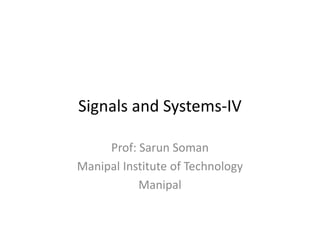
Time Property Periodic Non periodic
Continuous
(t)
Fourier Series
(FS)
Fourier Transform
(FT)
Discrete
[n]
Discrete Time Fourier Series
(DTFS)
Discrete Time Fourier Transform
(DTFT)
Prof: Sarun Soman, MIT, Manipal 2](data:image/gif;base64,R0lGODlhAQABAIAAAAAAAP///yH5BAEAAAAALAAAAAABAAEAAAIBRAA7)
Recommandé
Contenu connexe
Tendances
Tendances (20)
Similaire à Signals and systems-4
Similaire à Signals and systems-4 (20)
Dernier
Dernier (20)
Signals and systems-4
- 1. Signals and Systems-IV Prof: Sarun Soman Manipal Institute of Technology Manipal
- 2. Fourier Representations of Signals and LTI Systems Time Property Periodic Non periodic Continuous (t) Fourier Series (FS) Fourier Transform (FT) Discrete [n] Discrete Time Fourier Series (DTFS) Discrete Time Fourier Transform (DTFT) Prof: Sarun Soman, MIT, Manipal 2
- 3. Continuous Time Periodic Signals: Fourier Series FS of a signal x(t) ݔ ݐ = ܺ[݇]݁ఠబ௧ ஶ ୀିஶ )ݐ(ݔ fundamental period is T, fundamental frequency ߱ = ଶగ ் A signal is represented as weighted superposition of complex sinusoids. Representing signal as superposition of complex sinusoids provides an insightful characterization of signal. The weight associated with a sinusoid of a given frequency represents the contribution of that sinusoid to the overall signal. Prof: Sarun Soman, MIT, Manipal 3
- 4. Jean Baptiste Joseph Fourier (21 March 1768 – 16 May 1830) Prof: Sarun Soman, MIT, Manipal 4
- 5. Continuous Time Periodic Signals: Fourier Series Prof: Sarun Soman, MIT, Manipal 5
- 6. Continuous Time Periodic Signals: Fourier Series ܺ ݇ − Fourier Coefficient ܺ ݇ = 1 ܶ න ݁)ݐ(ݔିఠబ௧݀ݐ ் Fourier series coefficients are known as a frequency –domain representation of .)ݐ(ݔ Eg. Determine the FS representation of the signal. ݔ ݐ = 3 cos గ ଶ ݐ + గ ସ using the method of inspection. Prof: Sarun Soman, MIT, Manipal 6
- 7. Example ܶ = 4, ߱ = ߨ 2 FS representation of a signal x(t) ݔ ݐ = ܺ[݇]݁ఠబ௧ ஶ ୀିஶ ݔ ݐ = ܺ[݇]݁ గ ଶ ௧ ஶ ୀିஶ (1) Using Euler’s formula to expand given .)ݐ(ݔ ݔ ݐ = 3 ݁ గ ଶ௧ା గ ସ + ݁ ି గ ଶ௧ା గ ସ 2 )ݐ(ݔ = 3 2 ݁ గ ସ݁ గ ଶ ௧ + 3 2 ݁ି గ ସ݁ି గ ଶ ௧ (2) Equating each term in eqn (2) to the terms in eqn (1) X k = 3 2 eି୨ ସ, k = 1 3 2 e୨ ସ, k = −1 0, otherwise Prof: Sarun Soman, MIT, Manipal 7
- 8. Example All the power of the signal is concentrated at two frequencies ࣓ = ࣊ and ࣓ = − ࣊ . Determine the FS coefficients for the signal )ݐ(ݔ Ans: ܶ = 2, ߱ = ߨ Magnitude & Phase Spectra t -2 0 2 4 6-1 x(t) ݁ିଶ௧ Prof: Sarun Soman, MIT, Manipal 8
- 9. Example ܺ ݇ = 1 ܶ න ݁)ݐ(ݔିఠబ௧݀ݐ ் ܺ ݇ = 1 2 න ݁ିଶ௧݁ିగ௧݀ݐ ଶ = 1 2 න ݁ି(ଶାగ)௧݀ݐ ଶ ܺ ݇ = −1 2(2 + ݆݇ߨ) ݁ି(ଶାగ)௧ | ଶ = 1 4 + ݆2݇ߨ 1 − ݁ିସ݁ିଶగ ݁ିଶగ = 1 = 1 − ݁ିସ 4 + ݆݇2ߨ Find the time domain signal whose FS coefficients are ܺ ݇ = ݆ߜ ݇ − 1 − ݆ߜ ݇ + 1 + ߜ ݇ − 3 + ߜ ݇ + 3 , ߱ = ߨ Ans: FS of a signal x(t) ݔ ݐ = ܺ[݇]݁ఠబ௧ ஶ ୀିஶ ݔ ݐ = ܺ[݇]݁గ௧ ஶ ୀିஶ = ݆݁(ଵ)గ௧ − ݆݁(ିଵ)గ௧ + ݁(ଷ)గ௧ + ݁(ିଷ)గ௧ Prof: Sarun Soman, MIT, Manipal 9
- 10. Example = ݆(2݆ sin ߨ)ݐ + 2 cos 3ߨݐ = − ܖܑܛ ࢚࣊ + ܛܗ܋ ࢚࣊ Find the FS coefficient of periodic signal )ݐ(ݔ as shown in Fig. Ans: ܶ = 6, ߱ = ߨ 3 ܺ ݇ = 1 ܶ න ݁)ݐ(ݔିఠబ௧݀ݐ ் ଶ ି ் ଶ ܺ ݇ = 1 6 න ݁)ݐ(ݔି గ ଷ ௧ ݀ݐ ଷ ିଷ = 1 6 න 1 ݁ି గ ଷ௧ ݀ݐ + න (−1) ଶ ଵ ିଵ ିଶ ݁ି గ ଷ ௧ ݀ݐ = 1 6 ݁ି గ ଷ ௧ −݆݇ ߨ 3 |ିଶ ିଵ + ݁ି గ ଷ ௧ ݆݇ ߨ 3 |ଵ ଶ 0 2 4-2 -4 t x(t) Prof: Sarun Soman, MIT, Manipal 10
- 11. Example = 1 6 ݁ି గ ଷ(ିଶ) − ݁ି గ ଷ(ିଵ) ݆݇ ߨ 3 + ݁ି గ ଷ(ଶ) − ݁ି గ ଷ(ଵ) ݆݇ ߨ 3 = 1 6 ݁ ଶగ ଷ + ݁ି ଶగ ଷ ݆݇ ߨ 3 − ݁ గ ଷ + ݁ି గ ଷ ݆݇ ߨ 3 = 1 ݆2ߨ݇ 2 ܿݏ 2ߨ݇ 3 − 2 cos ߨ݇ 3 , ݇ ≠ 0 For ݇ = 0 ܺ 0 = 1 6 න ݐ݀)ݐ(ݔ ଷ ିଷ = 1 6 න 1 ݀ݐ + න (−1) ଶ ଵ ିଵ ିଶ ݀ݐ = 1 6 −1 + 2 − 1 = 0 The DC component is zero. Prof: Sarun Soman, MIT, Manipal 11
- 12. Example Find the FS coefficient of the signal .)ݐ(ݔ Ans: ܶ = 2, ߱ = ߨ ݔ ݐ = ൜ 1 + ,ݐ −1 < ݐ < 0 1 − ,ݐ 0 < ݐ < 1 ܺ ݇ = 1 ܶ න ݁)ݐ(ݔିఠబ௧ ݀ݐ ் ଶ ି ் ଶ ܺ ݇ = 1 2 න ݁)ݐ(ݔିగ௧݀ݐ ଵ ିଵ = 1 2 ቈන 1 + ݐ ݁ିగ௧ ݀ݐ ିଵ + න 1 + ݐ ݁ିగ௧݀ݐ ଵ = 1 2 ቈන 1 ݁ିగ௧ ݀ݐ ିଵ + න ݐ ݁ିగ௧ ݀ݐ ିଵ + න 1 ݁ିగ௧ ݀ݐ ଵ + න ݐ ݁ିగ௧ ݀ݐ ଵ 10-1-2 2 t x(t) Prof: Sarun Soman, MIT, Manipal 12
- 13. Example ܺ ݇ = 1 ߨଶ݇ଶ 1 − −1 , ݇ ≠ 0 For ݇ = 0 ܺ 0 = 1 2 ቈන (1 ିଵ + ݐ)݀ݐ + න 1 − ݐ ݀ݐ ଵ = 1 2 ܵ݅݊ܿ function ܿ݊݅ݏ ݑ = sin ߨݑ ߨݑ The functional form ୱ୧୬ గ௨ గ௨ often occurs in Fourier Analysis Prof: Sarun Soman, MIT, Manipal 13
- 14. Continuous Time Periodic Signals: Fourier Series – The maximum of the function is unity at ݑ = 0. – The zero crossing occur at integer values of .ݑ – Mainlobe- portion of the function b/w the zero crossings at ݑ = ±1. – Sidelobes- The smaller ripples outside the mainlobe. – The magnitude dies off as ଵ ௨ . Prof: Sarun Soman, MIT, Manipal 14
- 15. Continuous Time Periodic Signals: Fourier Series Determine the FS representation of the square wave depicted in Fig. Ans: The period is T , ߱ = ଶగ ் The signal has even symmetry, integrate over the range − ் ଶ ݐ ் ଶ ܺ ݇ = 1 ܶ න ݁)ݐ(ݔିఠబ௧݀ݐ ் ଶ ି ் ଶ ܺ ݇ = 1 ܶ න (1)݁ିఠబ௧݀ݐ ் ଶ ି ் ଶ ܺ ݇ = 1 ܶ න (1) ்ೞ ି்ೞ ݁ିఠబ௧݀ݐ ܺ ݇ = −1 ܶ݇߱ ݁ିఠబ௧|ି்ೞ ்ೞ ܺ ݇ = −1 ܶ݇߱ ݁ିఠబ்ೞ − ݁ఠబ்ೞ ܺ ݇ = 2 ܶ݇߱ ݁ఠబ்ೞ − ݁ିఠబ்ೞ ݆2 ܺ ݇ = 2 ܶ݇߱ sin ݇߱ܶ௦ , ݇ ≠ 0 Prof: Sarun Soman, MIT, Manipal 15
- 16. Example For ݇ = 0 ܺ 0 = 1 ܶ න ݀ݐ ்ೞ ି்ೞ = 2ܶ௦ ܶ ܺ ݇ = 2 ܶ݇߱ sin ݇߱ܶ௦ ߱ = 2ߨ ܶ ܺ ݇ = sin ߨ݇ 2ܶ௦ ܶ ߨ݇ ܺ ݇ = 2ܶ௦ ܶ sin ߨ݇ 2ܶ௦ ܶ ߨ݇ 2ܶ௦ ܶ ܺ ݇ = 2ܶ௦ ܶ ܿ݊݅ݏ ݇ 2ܶ௦ ܶ 2ܶ௦ ܶ = 1 8 = 12.5% 2ܶ௦ ܶ = 1 2 = 50% Prof: Sarun Soman, MIT, Manipal 16
- 17. Example Use the defining equation for the FS coefficients to evaluate the FS representation for the following signals. ݔ ݐ = sin 3ߨݐ + cos 4ߨݐ Ans: ܶଵ = 2 3 , ܶଶ = 1 2 )ݐ(ݔ will be periodic with T=2sec. Fundamental frequency ߱ = ߨ ݔ ݐ ݔ ݐ = ܺ[݇]݁ఠబ௧ ஶ ୀିஶ ܺ ݇ = 1 2 , ݇ = ±4 1 ݆2 , ݇ = 3 −1 ݆2 , ݇ = −3 Prof: Sarun Soman, MIT, Manipal 17
- 18. 0 x(t) t 2 1 3 2 3 4 3 − 8 3 -2 − 2 3 − 4 3 Example Find X[k] Ans: m x(t) 0 2δ(t) 1 −ߜ ݐ − 1 3 − ߜ ݐ + 2 3 2 ߜ ݐ − 2 3 + ߜ ݐ + 4 3 3 −ߜ ݐ − 1 − ߜ ݐ + 2 4 ߜ ݐ − 4 3 + ߜ ݐ + 8 3 1 Prof: Sarun Soman, MIT, Manipal 18
- 19. Example m x(t) -1 −ߜ ݐ + 1 3 − ߜ ݐ − 2 3 -2 ߜ ݐ + 2 3 + ߜ ݐ − 4 3 -3 −ߜ ݐ + 1 − ߜ ݐ − 2 -4 ߜ ݐ + 4 3 + ߜ ݐ − 8 3 -1 0 x(t) t 2 − 1 3 2 3 4 3 − 8 3 -2 − 2 3 − 4 3 1-1 0 x(t) t 2 − 1 3 1 3 4 3 -2 − 4 3 ܺ ݇ = 1 ܶ න ݁)ݐ(ݔିఠబ௧ ݀ݐ ் ଶ ି ் ଶ ܺ ݇ = 3 4 න ݁)ݐ(ݔି ଷగ ଶ ௧ ݀ݐ ଶ ଷ ି ଶ ଷ Prof: Sarun Soman, MIT, Manipal 19
- 20. Example ܺ ݇ = 3 4 න 2δ t − δ t − 1 3 − δ t + 1 3 ݁ି ଷగ ଶ ௧ ݀ݐ ଶ ଷ ି ଶ ଷ Using sifting property ܺ ݇ = 3 4 2 − ݁ି గ ଶ − ݁ గ ଶ ܺ ݇ = 6 4 − 6 4 cos ݇ ߨ 2 Prof: Sarun Soman, MIT, Manipal 20
- 21. Discrete Time Periodic Signals: The Discrete Time Fourier Series DTFS representation of a periodic signal with fundamental frequency Ω = ଶగ ே ݔ ݊ = ܺ[݇]݁Ωబ ேିଵ ୀ Where ܺ ݇ = 1 ܰ ]݊[ݔ ேିଵ ୀ ݁ିΩబ Prof: Sarun Soman, MIT, Manipal 21
- 22. Discrete Time Periodic Signals: The Discrete Time Fourier Series ]݊[ݔand ܺ ݇ are exactly characterized by a finite set of N numbers. DTFS is the only Fourier representation that can be numerically evaluated and manipulated in a computer. ݔ ݊ is ‘N’ periodic in ‘n’ ܺ[݇] is ‘N’ periodic in ‘k’ Prof: Sarun Soman, MIT, Manipal 22
- 23. Example Find the frequency domain representation of the signal depicted in Fig. Ans: ܰ = 5, Ω = 2ߨ 5 ܺ ݇ = 1 ܰ ]݊[ݔ ேିଵ ୀ ݁ିΩబ The signal has odd symmetry, sum over n=-2 to 2 ܺ ݇ = 1 5 ]݊[ݔ ଶ ୀିଶ ݁ି ଶగ ହ = 1 5 ൜0 + 1 2 ݁ ଶగ ହ + 1 − 1 2 ݁ି ଶగ ହ + 0ൠ = 1 5 1 + ݆ sin 2ߨ݇ 5 ● 1 ●● -2 0 2 -4 y[n] n4 -6 ● ●6● 1 2ൗ Prof: Sarun Soman, MIT, Manipal 23
- 24. Example X[k] will be periodic with period ‘N’. Values of X[k] for k=-2 to 2. Calculator in radians mode ܺ −2 = 1 5 1 − ݆ sin 4ߨ 5 = 0.232݁ି.ହଷଵ ܺ −1 = 1 5 1 − ݆ sin 2ߨ 5 = 0.276݁ି. ܺ 0 = 1 5 ܺ 1 = 1 5 1 + ݆ sin 2ߨ 5 = 0.276݁. ܺ 2 = 1 5 1 + ݆ sin 4ߨ 5 = 0.232݁.ହଷଵ Mag & phase plot. Prof: Sarun Soman, MIT, Manipal 24
- 25. Example Use the defining equation for the DTFS coefficients to evaluate the DTFS representation for the following signals. ݔ ݊ = cos 6ߨ 17 ݊ + ߨ 3 ݔ ݊ = ܺ[݇]݁Ωబ ேିଵ ୀ ܰ = 17, Ω = 2ߨ 17 ݔ ݊ = 1 2 ݁ గ ଵା గ ଷ + ݁ ି గ ଵା గ ଷ ݔ ݊ = 1 2 ݁ గ ଷ݁(ଷ) ଶగ ଵ + 1 2 ݁ି గ ଷ݁(ିଷ) ଶగ ଵ ܺ[݇] = 1 2 ݁ గ ଷ, ݇ = 3 1 2 ݁ି గ ଷ, ݇ = −3 0, ݇ ݊ ݁ݏ݅ݓݎ݄݁ݐ = {−8, −7, … , 8} Prof: Sarun Soman, MIT, Manipal 25
- 26. Example ݔ ݊ = 2 sin 4ߨ 19 ݊ + cos 10ߨ 19 ݊ + 1 Ans: ܰ = 19, Ω = 2ߨ 19 = 1 ݆ ݁ ସగ ଵଽ − ݁ି ସగ ଵଽ + 1 2 ݁ ଵగ ଵଽ + ݁ି ଵగ ଵଽ + 1 = −݆݁ ଶ ଶగ ଵଽ + ݆݁ ିଶ ଶగ ଵଽ + 1 2 ݁ ହ ଶగ ଵଽ + 1 2 ݁ ିହ ଶగ ଵଽ + 1݁ ଶగ ଵଽ ݔ ݊ = ܺ[݇]݁Ωబ ேିଵ ୀ ܺ ݇ = 1 2 , ݇ = ±5 ݆, ݇ = −2 1, ݇ = 0 −݆, ݇ = 2 0, ݇ ݊ ݁ݏ݅ݓݎ݄݁ݐ = {−9,8, . . , 9} Prof: Sarun Soman, MIT, Manipal 26
- 27. Example ݔ ݊ = [ −1 (ߜ ݊ − 2݉ ஶ ୀିஶ + ߜ ݊ + 3݉ )] Ans ܰ = 12, Ω = ߨ 6 ܺ ݇ = 1 ܰ ]݊[ݔ ேିଵ ୀ ݁ିΩబ m x[n] 0 2ߜ[݊] 1 −ߜ ݊ − 2 − ߜ[݊ + 3] 2 ߜ ݊ − 4 + ߜ[݊ + 6] 3 −ߜ ݊ − 6 − ߜ[݊ + 9] 4 ߜ ݊ − 8 + ߜ[݊ + 12] 5 −ߜ ݊ − 10 − ߜ[݊ + 15] 6 ߜ ݊ − 12 + ߜ[݊ + 18] m x[n] -1 −ߜ ݊ + 2 − ߜ[݊ − 3] -2 ߜ ݊ + 4 + ߜ[݊ − 6] -3 −ߜ ݊ + 6 − ߜ[݊ − 9] -4 ߜ ݊ + 8 + ߜ[݊ − 12] -5 −ߜ ݊ + 10 − ߜ[݊ − 15] -6 ߜ ݊ + 2 + ߜ[݊ − 18] Prof: Sarun Soman, MIT, Manipal 27
- 28. Example ܺ ݇ = 1 12 ]݊[ݔ ୀିହ ݁ି గ ݔ ݊ = 0, ݂݊ ݎ = ±5,6 Prof: Sarun Soman, MIT, Manipal 28
- 29. Example ݔ ݊ = cos ݊ߨ 30 + 2 sin ݊ߨ 90 Ans: Ωଵ = ߨ݊ 30 = 2ߨ݊ 60 ܰଵ = 60, ܰଶ = 180 ܰଵ ܰଶ = 1 3 ݔ ݊ will be periodic with period N=180, Ω = ଶగ ଵ଼ ݔ ݊ = 1 2 ݁ గ ଷ + ݁ି గ ଷ + 1 ݆ ݁ గ ଽ − ݁ି గ ଽ ݔ ݊ = ܺ[݇]݁Ωబ ேିଵ ୀ ݔ ݊ = 1 2 ݁(ଷ) ଶగ ଵ଼ + ݁(ିଷ) ଶగ ଵ଼ − ݆ ݁(ଵ) ଶగ ଵ଼ − ݁(ିଵ) ଶగ ଵ଼ ܺ ݇ = ݆, ݇ = −1 −݆, ݇ = 1 1 2 , ݇ = ±3 0, ݊ ݁ݏ݅ݓݎ݄݁ݐ − 89 ≤ ݇ ≤ 90 Prof: Sarun Soman, MIT, Manipal 29
- 30. Example Inverse DTFS: used to determine the time domain signal x[n] from DTFS coefficients X[k]. Ans: ܰ = 9, Ω = 2ߨ 9 Take ݇ = −4 4 ݐ Find ܺ[݇]from the plot. ݔ ݊ = ܺ[݇]݁Ωబ ேିଵ ୀ ݔ ݊ = ܺ[݇]݁ ଶగ ଽ ସ ୀିସ ࡷ ࢄ[] -4 0 -3 ݁ ଶగ ଷ -2 2݁ గ ଷ -1 0 0 ݁గ 1 0 2 2݁ି గ ଷ 3 ݁ି ଶగ ଷ 4 0 Prof: Sarun Soman, MIT, Manipal 30
- 31. Example ݔ ݊ = ݁ ଶగ ଷ ݁(ିଷ) ଶగ ଽ + 2݁ గ ଷ݁(ିଶ) ଶగ ଽ + ݁గ݁() ଶగ ଽ + 2݁ି గ ଷ݁(ଶ) ଶగ ଽ + ݁ି ଶగ ଷ ݁(ଷ) ଶగ ଽ ݔ ݊ = 2 cos 6ߨ݊ 9 − 2ߨ 3 + 4 sin 4ߨ݊ 9 − ߨ 3 − 1 Find x[n]. Ans: ܰ = 12, Ω = 2ߨ 12 Prof: Sarun Soman, MIT, Manipal 31
- 32. Example ݔ ݊ = ܺ[݇]݁ ଶగ ଵହ ସ ୀିସ From table expression for ܺ[݇] ܺ ݇ = ݁ି గ ݔ ݊ = ݁ି గ ݁ ଶగ ଵହ ସ ୀିସ ݔ ݊ = ݁ గ ଶ ଵହ ି ଵ ସ ୀିସ Let ݈ = ݇ + 4 ݔ ݊ = ݁ గ ଶ ଵହ ି ଵ ିସ ଼ ୀ ࢄ[] -4 ݁ ସగ -3 ݁ ଷగ -2 ݁ ଶగ -1 ݁ గ 0 1 1 ݁ି గ 2 ݁ି ଶగ 3 ݁ି ଷగ 4 ݁ି ସగ Prof: Sarun Soman, MIT, Manipal 32
- 33. Example ݔ ݊ = ݁ ିସగ ଶ ଵଶ ି ଵ ݁ గ ଶ ଵଶ ି ଵ ଼ ୀ ݔ ݊ = ݁ ିସగ ଶ ଵଶି ଵ 1 − ݁ ଽగ ଶ ଵଶ ି ଵ 1 − ݁ గ ଶ ଵଶି ଵ Prof: Sarun Soman, MIT, Manipal 33
- 34. Example = ݁ ିସగ ଶ ଵଶି ଵ ݁ ଽ ଶగ ଶ ଵଶି ଵ ݁ ି ଽ ଶగ ଶ ଵଶି ଵ − ݁ ଽ ଶగ ଶ ଵଶି ଵ ݁ గ ଶ ଶ ଵଶ ି ଵ ݁ ି గ ଶ ଶ ଵଶ ି ଵ − ݁ గ ଶ ଶ ଵଶ ି ଵ = ݁ ି ଽ ଶగ ଶ ଵଶି ଵ − ݁ ଽ ଶగ ଶ ଵଶି ଵ ݁ ି గ ଶ ଶ ଵଶି ଵ − ݁ గ ଶ ଶ ଵଶି ଵ = sin 9 2 ߨ 2݊ 12 − 1 6 sin ߨ 2 2݊ 12 − 1 6 Prof: Sarun Soman, MIT, Manipal 34