1. THERMODYNAMICS OF BIOLOGICAL SYSTEMS
LESSON 10:
CALCULATION OF FLOW PROCESSES BASED ON ACTUAL PROPERTY CHANGES
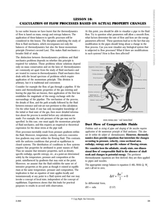
In our earlier lessons we have learnt that the thermodynamics At this point, you should be able to visualize a pipe to the fluid
of flow is based on mass, energy and entropy balances. The flow. Try to question what parameters will allow a smooth flow,
application of these balances to specific processes will be what factors determine the rate of flow and how are the energy
considered in this lesson. The discipline underlying the study of parameters affected. These questions lead us to the fact that any
flow is fluid mechanics, which encompasses not only the modification in the pipes should bring about a change in the
balances of thermodynamics but also the linear-momentum flow process. Can you now visualize any biological system that
principle (Newton’s second Law). This makes fluid mechanics a is subjected to flow processes? What if there are modifications
broader field of study. in such systems? How is flow then affected?
The distinction between thermodynamics problems and fluid
mechanics problems depends on whether this principle is
required for solution. Those problems whose solutions depend
only on mass conservation and on the laws of thermodynamics
are commonly set apart from the study of fluid mechanics and
are treated in courses in thermodynamics. Fluid mechanics then
deals with the broad spectrum of problems which require
application of the momentum principle. This division is
arbitrary, but it is traditional and convenient.
Consider for example the flow of gas through a pipeline. If the
states and thermodynamic properties of the gas entering and
leaving the pipe line are known, then application of the first law
establishes the magnitude of the energy exchange with the
surroundings of the pipeline. The mechanism of the process,
the details of flow, and the path actually followed by the fluid
between entrance and exit are not pertinent to this calculation.
On the other hand, if one has only incomplete knowledge of
the initial or final state of the gas, then more detailed informa-
tion about the process is needed before any calculations are
made. For example, the exit pressure of the gas may not be
www.rnceus.com/ vsd/norm.html
specified. In this case, one must apply the momentum principle
of fluid mechanics, and this requires an empirical or theoretical Duct Flow of Compressible Fluids
expression for the shear stress at the pipe wall. Problems such as sizing of pipes and shaping of the nozzles requires
Flow processes inevitably result from pressure gradients within application of the momentum principle of fluid mechanics. This does
the fluid. Moreover, temperature, velocity, and even concentra- not lie within the subject of thermodynamics. However, thermody-
tion gradients may exist within the flowing fluid. This contrasts namics does provide equations that interrelate the changes
with the uniform conditions that prevail at equilibrium in occurring in pressure, velocity, cross-sectional area,
closed systems. The distribution of conditions in flow systems enthalpy, entropy and specific volume of flowing stream.
requires that properties be attributed to point masses of fluid. We consider here the adiabatic, steady-state, one-dimen-
Thus we assume that intensive properties, such as density, sional flow of compressible fluid in the absence of shaft
specific enthalpy, specific entropy, etc., at a point are determined work and changes in potential energy. The pertinent
solely by the temperature, pressure and composition at the thermodynamic equations are first derived; they are then applied
point, uninfluenced by gradients that may exist at the point. to pipes and nozzles.
Moreover, we assume that the fluid exhibits the same set of The appropriate energy balance is equation (1-46). With Q, Ws
intensive properties at the point as though it existed at equilib- and z all set to zero,
rium at the same temperature, pressure and composition. The
implication is that an equation of state applies locally and ∆u 2
instantaneously at any point in a fluid system and that one may ∆H + =0
invoke a concept of local state, independent of the concept of 2
equilibrium. Experiences shows that this leads for practical In differential form,
purposes to results in accord with observation.
dH = -udu (2-57)
© Copy Right: Rai University
2.202 39

2. The continuity equation, (1-41), is also applicable. Since m. is
THERMODYNAMICS OF BIOLOGICAL SYSTEMS
(1 − M )VdP + 1 + βu 
2
constant, its differential form is: u2
2

 TdS −
 dA = 0 (2-61)
d(uA/V) = 0 C P  A
dV du dA where M is the Mach number, defined as the ratio of the
Or − − =0 (2-58) fluid in the duct to the speed of sound in the fluid, u/c.
V u A
Equation (2-61) relates dP to dS and dA.
The fundamental property relation appropriate to this applica-
Equation 2-60 and 2-61 are combined to eliminate VdP:
tion is:
dH = TdS + VdP  βu 2 
In addition, the specific volume of the fluid may be considered  +M2 
 CP   1 u
2
a function of its entropy and pressure: udu −  TdS +   dA = 0
1− M 2 1− M  A
2
(2-62)
V = V (s,p).  
 
 
 ∂V   ∂V 
Then, dV =   dS +   dP This equation relates to dS and dA. Combined with eq 2-57 it
 ∂S  P  ∂P  S relates dH to dS and dA, and combined with 2-58 it relates dV
This equation is put into more convenient form through the to these same independent variables.
mathematical identity: The differentials in the preceding equations represent changes in
the fluid as it traverses a differential length of its path. If this
 ∂V   ∂V   ∂T  length is dx, then each of the equations of flow may be divided
  =   
 ∂S  P  ∂T  P  ∂S  P through by dx. Equations 7.7 and 7.8 then become:
( ) dP + T 1 + βu  dS u 2 dA
2
Substituting for the two partial derivatives on the right by eqs.
V 1− M 2 
 
 dx − A dx = 0 (2-63)
 ∂S  C dx  C P 
2.3 and gives:   = P
 ∂T  P T
 βu 2 
 +M2 
  dS  1  u dA
2
 ∂V  βVT du
−T
CP
  =
u
dx 1− M 2  dx +  1 − M 2


 A dx
=0
(2-64)
where is the volume expansivity
 ∂S  P Cp 
 

 
According to the second law, the irreversibilities due to fluid
The equation derived in physics for the speed of sound c in a friction in adiabatic flow cause an entropy increase in the fluid in
fluid is: the direction of flow. In the limit as the flow approaches
reversibility, this increase approaches zero. In general, then,
 ∂P   ∂V  V 2 
c 2 = −V 2   or   = − 2 
c  dS
 ∂V  S  ∂P  S   ≥0
dx
substituting for the two partial derivatives in the equation for Pipe Flow
dV now yields: For the case of steady-state adiabatic flow in a horizontal
pipe of constant cross-sectional area, dA/dx = 0, and eqn..
dV βT V 2-63 and 2-64 reduces to:
= dS − 2 dP (2-59)
V CP c
 βu 2   βu 2 
Equations 2-57, 2-58, 2-48 and 2-59 relate the six differentials- 1+   +M 2 
dH, du, dv, dA, dS, and dP. With but four equations, we treat dP T CP  dS du  CP  dS
=−   dx u dx = T  1 − M 2  dx
dS and dA as independent, and develop equations that express dx V 1− M 2
   
the remaining differentials as functions of these two. First, eqns    
2-57 and 2-48 are combined:    
TdS + VdP = -udu (2-60)
For subsonic flow, M2 < 1, and all quantities on the right sides
Eliminating dV and du from eqs. 2-58 by eqs. 2-59 and 2-60 dP
gives upon rearrangement: of these equations are positive whence, dx
<0
du
and >0
dx
© Copy Right: Rai University
40 2.202

3. Thus the pressure decreases and the velocity increases in the
THERMODYNAMICS OF BIOLOGICAL SYSTEMS
direction of flow. However, the velocity cannot increase
indefinitely. If the velocity were to exceed the sonic value, then
the above inequalities would reverse. Such a transition is not
possible in a pipe of constant cross-sectional area. For subsonic
flow, the maximum fluid velocity obtainable in a pipe of
constant cross section is the speed of sound, and this value is
reached at the exit of the pipe. At this point dS/dx reaches its
limiting value of zero. Given a discharge pressure low enough
for the flow to become sonic, lengthening the pipe does not
alter this result; the mass rate of flow decreases so that the sonic
velocity is still obtained at the outlet of the lengthened pipe.
The equations for pipe flow indicate that when flow is super-
sonic the pressure increases and the velocity decreases in the
direction of flow. However, such a flow regime is unstable, and
when a supersonic stream enters a pipe of constant cross
section, a compression shock occurs, the result of which is an
abrupt and finite increase in pressure and decrease in velocity to
a subsonic value.
The limitations observed for flow in pipes do not extend to
properly designed nozzles, which bring about the interchange
of internal and kinetic energy of a fluid as the result of a
changing cross-sectional area available for flow. The relation
between nozzle length and cross-sectional area is not susceptible
to thermodynamics analysis, but is a problem in fluid mechan-
ics. In a properly designed nozzle the area changes with length
in such a way as to make the flow nearly frictionless.
Problems
1. Consider the steady-state, adiabatic, irreversible flow flow of
an incompressible liquid in a horizontal pipe of constant
cross-sectional area. Show that:
a. The velocity is constant
b. The temperature increases in the direction of flow
c. The pressure decreases in the direction of flow
References
1. J. M. Smith, H. C. Van Ness, M. M. Abbott, Adapted by B.
I. Bhatt, Introduction To Chemical Engineering
Thermodynamics, Sixth Edition, Tata McGraw-Hill
Publishing Company Ltd, New Delhi
Notes
© Copy Right: Rai University
2.202 41