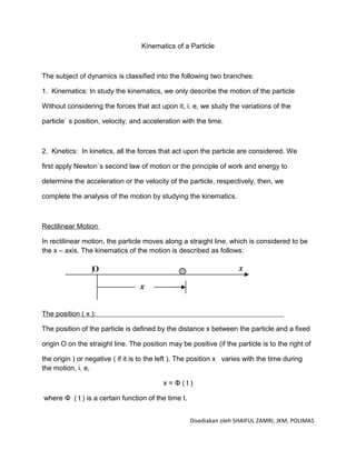
1. Kinematics of a Particle
The subject of dynamics is classified into the following two branches:
1. Kinematics: In study the kinematics, we only describe the motion of the particle
Without considering the forces that act upon it, i. e, we study the variations of the
particle` s position, velocity, and acceleration with the time.
2. Kinetics: In kinetics, all the forces that act upon the particle are considered. We
first apply Newton`s second law of motion or the principle of work and energy to
determine the acceleration or the velocity of the particle, respectively, then, we
complete the analysis of the motion by studying the kinematics.
Rectilinear Motion
In rectilinear motion, the particle moves along a straight line, which is considered to be
the x – axis. The kinematics of the motion is described as follows:
The position ( x ):
The position of the particle is defined by the distance x between the particle and a fixed
origin O on the straight line. The position may be positive (if the particle is to the right of
the origin ) or negative ( if it is to the left ). The position x varies with the time during
the motion, i. e,
x=Φ(t)
where Φ ( t ) is a certain function of the time t.
Disediakan oleh SHAIFUL ZAMRI, JKM, POLIMAS

2. The velocity ( v ):
The instantaneous velocity of the particle ( its velocity at any instant ) is defined by the
rate of change of its position with respect to the time, i. e,
V=
The acceleration ( a ):
It is defined as the time rate of change of the particle`s velocity, i. e,
a=
In some cases, as we will see later, it will be necessary to substitute the acceleration in
the following mathematical form:
Which is derived as follows :
The displacement ( ∆ x ) :
The displacement of a particle during a certain time interval is defined as the change of
its position. If at a certain instant ti the corresponding position is xi and at another
instant tf ( tf > ti ) the corresponding position is xf then, the displacement that happened
Disediakan oleh SHAIFUL ZAMRI, JKM, POLIMAS

3. during the time interval ( ∆t = tf – ti ) will be ∆x = xf – xi. The displacement ∆x may be
positive or negative.
The distance traveled ( D ) :
The distance traveled during a time interval ∆t is defined by the total length of the path
over which the particle travels. To determine the distance traveled during a certain time
interval ∆t from t = ti up to t = tf, the following steps must be followed:
a- determine the position xi that corresponds to ti and xf that corresponds to xf.
b- substitute v = 0 into the relation ( v , t ) to determine the solutions of this algebraic
equation ( v = 0 ) , say t1 , t2,….
c- determine the corresponding positions that correspond to the instants t 1, t2 , …, that
are contained inside the time interval ∆t.
d- plot, on the straight line, the values of the position x that correspond to the instants
ti , tf, t1, …as shown and calculate the path length between each two successive
instants.
D = d1 + d2 + d3.
Types of applications:
1. Differentiation problems:
Given: The relation between the position and the time ( x , t ).
Disediakan oleh SHAIFUL ZAMRI, JKM, POLIMAS

4. Required: The velocity v and the acceleration f at any instant.
Method of solution: By differentiating ( x , t ) we obtain (v , t ), then differentiating ( v ,
t ), we obtain ( a , t ).
Example ( 1 ):
A particle is moving along a straight line such that its position is given by :
x = t3 – 6t2+ 9t m, where t is in seconds. Determine the distance traveled during the
first 2 seconds.
Disediakan oleh SHAIFUL ZAMRI, JKM, POLIMAS

5. 2. Integration problems:
In the integration problems, the acceleration is given and the required is the position ( x
, t ), then we must execute two integration steps. To determine the constants of
integration, additional data must be given. Almost the initial conditions x 0 , v0 are
given. According to the given data of the problem, the integration problems are
classified into four cases :
a – Given: ( a , t ) and the initial conditions x 0 , v0.
Required: ( x , t )
Method of solution: substitute a = dv / dt in the relation ( a , t ) , the first integration
step results in ( v , t ) , then substitute v = dx / dt in the relation ( v , t ) and integrate
again , the relation ( x , t ) will be obtained. Example ( 2 )
b- Given : ( a , x ) + v0 , x0
Required: ( x , t )
Method of solution : substitute a = vdv / dx in the relation ( a , x ), the first integration
step will result in ( v , x ), then substitute v = dx / dt in the relation ( v , x ) and integrate
again , the relation ( x , t ) will be obtained. Example ( 3 )
c: Given : ( a , v ) + v0 , x0
Required : ( x , t )
Solution : substitute a = dv/dt or a = vdv/dx according to the required relations and
integrate twice to obtain ( x , t ). Example ( 4 )
d – Given : a = constant + v 0 , x0
Required : ( v , t ) , ( x , t ) or/and ( x , t )
Disediakan oleh SHAIFUL ZAMRI, JKM, POLIMAS

6. Solution : substitute directly in the following relations of constant acceleration
motion : Example ( 5 )
Example ( 2 ) :
A particle moves along a straight line such that its acceleration is given by:
a = 2t – 6 m / s2, where t is in seconds. If the motion is started from the origin with a
velocity of 5 m / sec., determine the distance it travels during the first 6 seconds.
Disediakan oleh SHAIFUL ZAMRI, JKM, POLIMAS

7. Example ( 3 ) :
A car starts from rest and moves along a straight line with an acceleration of
a = 3x-1/3 m/s2, where x is in meters. Determine the velocity and the position of the car
after 6 seconds.
Solution:
Disediakan oleh SHAIFUL ZAMRI, JKM, POLIMAS

8. Example ( 4 ) :
A particle is moving along a straight line such that it starts from the origin with a velocity
of 4 m / sec. If it begins to decelerate at the rate of a = - 2v m / s 2, where v is in m / s,
determine the distance it travels before it stops.
Solution :
Disediakan oleh SHAIFUL ZAMRI, JKM, POLIMAS

9. Example ( 5 ) :
A car has an initial velocity of 25 m/s and moves with a constant deceleration of 3
m/s2. Determine the velocity of the car after 4 seconds. What will be the displacement
of the car during this time interval .
Solution :
Disediakan oleh SHAIFUL ZAMRI, JKM, POLIMAS

10. Example (6 ):
A particle moves along a straight line with an acceleration a = - 4x m/s 2 where x is in
meters. The initial conditions of the motion are : x0 = 0 , v0 = 4 m/s. Find the relations
( v , t ) , ( x , t ).
Solution :
Disediakan oleh SHAIFUL ZAMRI, JKM, POLIMAS

11. RECTILINEAR KINEMATICS: ERRATIC MOTION
When a particle has a erratic or changing motion then its position, velocity and acceleration
cannot be described by a single
S-T GRAPH
• Plots of position vs. time can be used to find
velocity vs. time curves. Finding the slope of the
line tangent to the motion curve at any point is
the velocity at that point
v = ds/dt
slope of S-T graph = velocity
• Therefore, the v-t graph can be constructed by
finding the slope at various points along the s-t
graph.
• For example, by measuring the slope on the S-T
graph when t=t1, the velocity is v1, which is
plotted in Fig. The graph can be constructed by
plotting this and other value at each instant
Disediakan oleh SHAIFUL ZAMRI, JKM, POLIMAS

12. V-T GRAPH
• Plot of velocity vs. time can be used to fine
acceleration vs. time curves. Finding the
slope of the line tangent to velocity at any
point is the acceleration at that point
a = dv/dt
slope of S-T graph = velocity
• Therefore, the acceleration vs. time (or a-t)
graph can be constructed by finding the
slope at various points along the v-t graph
A-T GRAPH
Disediakan oleh SHAIFUL ZAMRI, JKM, POLIMAS

13. • Given the acceleration vs. time or a-t curve, the
change in velocity (∆v) during a time period is
the area under the a-t curve.
∆v =
Change in velocity = are under a-t graph
• So we can construct a v-t graph from an a-t
graph if we know the initial velocity of the
particle.
A-S GRAPH
• A more complex case is presented by the acceleration
versus position or a-s graph. The area under the a-s
curve represents the change in velocity
(recall a ds = v dv ).
• This equation can be solved for v1, allowing you to
solve for the velocity at a point. By doing this
repeatedly, you can create a plot of velocity versus
distance.
V-S GRAPH
Disediakan oleh SHAIFUL ZAMRI, JKM, POLIMAS

14. • Another complex case is presented by the velocity vs.
distance or v-s graph. By reading the velocity v at a point on
the curve and multiplying it by the slope of the curve (dv/ds)
at this same point, we can obtain the acceleration at that
point. Recall the formula
a = v (dv/ds).
• Thus, we can obtain an a-s plot from the v-s curve.
EXAMPLE 5
A bicycle moves along a straight road such
That its position is described by the graph
Show in fig. Construct the v-t and a-t for
0≤ t ≤30s
Disediakan oleh SHAIFUL ZAMRI, JKM, POLIMAS

15. EXAMPLE 6
Disediakan oleh SHAIFUL ZAMRI, JKM, POLIMAS

16. EXAMPLE 7
Disediakan oleh SHAIFUL ZAMRI, JKM, POLIMAS