Le document traite de l'analyse de la régression linéaire simple, en mettant l'accent sur des concepts tels que la minimisation des erreurs, l'estimation des coefficients et l'évaluation de la corrélation entre les variables. Il présente également des formules essentielles comme celle de la somme des carrés et décrit le coefficient de détermination (r²) pour quantifier la variation expliquée. Enfin, il aborde l'intervalle de confiance de la pente pour déterminer la significativité des relations entre les variables.

3. Les hypothèses à vérifier

4. Analyse des régression linéaires
simple
alors...?
.
possible..
petit
plus
le
être
doit
D
2
1
1
2
2
2
1
1
2
b
a,
b
a,
)
(
:
est
droite
la
à
écarts
des
carrés
des
somme
la
,....,
1
,
:
aux
les
liant
suivante
équation
l'
et
,...,
,
:
ns
observatio
a
on
l'
Si
.
aux
méthode
la
à
correspond
2
critère
Le
min
.
2
min
1.
:
és
possibilit
Plusieurs
minimiser
faut
Il
i
i
n
i
n
i
i
i
i
i
i
i
n
n
i i
i i
i
i
i
i
ax
b
y
D
n
i
ax
b
y
x
y
)
,y
(x
)
,y
(x
)
,y
(x
n
ax
b
y























carrés
moindres

5. Analyse des régression linéaires simple
 
 
bien...
ou
0
0
:
par
données
sont
de
et
de
estimées
valeurs
Les
)
(
2
)
(
2
)
(
zéro.
à
égales
pose
les
on
et
partielles
dérivées
...
n
1
i
n
1
i
1
1
1
2































i
i
i
i
i
n
i
i
i
i
n
i
i
i
n
i
i
i
ax
b
y
x
ax
b
y
b
a
ax
b
y
x
a
D
ax
b
y
b
D
ax
b
y
D

6. Analyse des régression linéaires
simple










































n
i
i
n
n
i
i
n
n
i
i
n
i
i
i
n
i
i
n
i
i
n
i
i
n
i
i
n
i
i
i
n
i
i
n
i
i
n
i
i
n
y
n
y
y
y
n
x
n
x
x
x
x
a
x
b
y
x
x
a
nb
y
x
a
x
b
y
x
x
a
nb
y
1
1
1
1
1
2
1
1
1
1
1
2
1
1
1
1
...
et
...
:
part
autre
D'
dire...
-
à
-
est
C'
0
0

8. exemple
Numéro de l'essai ‘X’ Masse ‘Y’ Longueur mi
2
mili
i mi li
1 2 42.0 4.0 84.0
2 4 48.4 16.0 193.6
3 6 51.3 36.0 307.8
4 8 56.3 64.0 450.4
5 10 58.6 100.0 586.0
n=5 30

 i
m 5
,
256

 i
l 220
2

 i
m 1622

 i
il
m
Balance à ressort
y = 2.055x + 38.99
30.0
35.0
40.0
45.0
50.0
55.0
60.0
65.0
0 2 4 6 8 10 12
Masse (kg)
Longueur
(cm)
  
 
38,99
2,055
















 
 

5
30
055
,
2
5
5
,
256
5
900
220
5
5
,
256
30
1622
2
2
n
m
a
n
l
b
n
m
m
n
l
m
l
m
a
i
i
i
i
i
i
i
i

9. 





2
2
)
(
2
)
ˆ
(
)
x
x
n
y
y
S(a
i
i
i
)]
(
);
(
[ )
2
,
2
/
(
)
2
,
2
/
( a
S
t
a
a
S
t
a
a n
n 
 

 

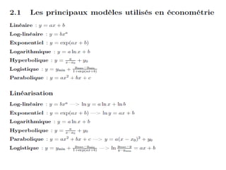
L’écart type de la pente a, estimé à partir de l’échantillon est noté S(a):
On peut alors déterminer l’intervalle de confiance de la pente (cf cours L1)
Si 0 apparaît dans cet intervalle, alors la pente ne peut être considérée comme
significativement différente de 0. On peut conclure qu’il n’existe pas de corrélation
significative entre les deux variables.
C’est l’ordonnée
estimée à partir du
modèle linéaire:

ˆ i
i
y ax b
 

10. Propriétés des estimateurs

11. Propriétés des estimateurs

12. Propriétés des estimateurs

13. Propriétés des estimateurs

20.     2
2
2
)
ˆ
(
ˆ y
y
y
y
y
y i
i
i
i 



 


Somme des carrés
totale (SCT)
Somme des carrés
des résidus (SCR)
Somme des carrés
de la régression (SCE)
Variation totale = variation inexpliquée + variation expliquée
R2 = Variation expliquée / variation totale
R2 est le coefficient de détermination, proportion de la variation
de y qui s’explique par la présence de x.
Plus R2 est grand, plus SCR est petit.

21. Coefficient de détermination
R2 =

2 2
2 2
2 2 2
ˆ
( ) *cov( , ) ( )
( ) ( ) ( )( )
i
i
y y X Y xy xy
y y V Y x x y y

 
 
  


2 2
1
( )
n
i y
i
SCT y y ns

  


22. Propriétés des estimateurs