1. Chapter 3: Solving Systems of Linear Equations
System of linear equations
a11x1 + a12x2 + ··· + a1nxn = b1
a21x1 + a22x2 + ··· + a2nxn = b2
. . .
. . .
an1x1 + an2x2 + ··· + annxn = bn
where aij and bi are some constant numbers, for i , j = 1, 2,..., n.
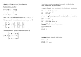
This system can be written in the matrix-vector form as: Ax = b
n
2
1
n
2
1
nn
n2
n1
2n
22
21
1n
12
11
b
b
b
b
,
x
x
x
x
,
a
a
a
a
a
a
a
a
a
A
Augmented matrix of the above linear system is given by
n
2
1
nn
n2
n1
2n
22
21
1n
12
11
b
b
b
a
a
a
a
a
a
a
a
a
or
b
|
A
Some linear systems in certain special forms can be solved easier than
others by using some specific procedures.
An upper triangular linear system can be solved by the back substitution.
(R1) a11x1 + a12x2 + a13x3 = b1
(R2) a22x2 + a23x3 = b2
(R3) a33x3 = b3
A lower triangular linear system can be solved by the forward substitution
(R1) a11x1 = b1
(R2) a21x1 + a22x2 = b2
(R3) a31x1 + a32x2 + a33x3 = b3
Example Solve the following linear systems.
(R1) 3x1+ x2+ x3 = 5
(R2) x2+ 2x3 = 4
(R3) 3x3 = 6
Example Solve the following linear systems.
(R1) 3x1 += 6
(R2) 2x1 + x2 = 4
(R3) 3x1 + x2 + x3 = 5
2. Elementary row operations
Elementary row operations are the following three rules for manipulating or
transforming an augmented matrix that leave the values of the solution set
unchanged.
1. Any two rows can be exchanged.
2. Any row may be multiplied (or divided) by a non-zero constant.
3. A multiple of any row can be added to any other row.
Example Show that the following two linear systems have the same solution.
(I) x - y = 2
2x - y - z = 3
x + y + z = 6
(II) x - y = 2
x - z = 1
3x - y + z = 10
Numerical methods for solving a system of linear equations
2 main types of methods for solving this linear system:
Direct methods
Give exact solution
Transform into the form that is easy to solve: i.e. either
upper triangular form,
lower triangular form, or
diagonal form
E.g. Gaussian Elimination upper triangular form
Gauss-Jordan diagonal form
LU decomposition upper and lower triangular form
Indirect methods or Iterative methods
Give approximate solution
Require initial approximate solution
E.g. Jacobi method
Gauss-Seidel method
3. Gaussian Elimination Method
Example: Solve the following system of linear equations by using Gaussian
elimination method.
x - y = 2
2x - y - z = 3
x + y + z = 6
Example - no solution
x - 2y - 6z = 12
x - 4y - 12z = 22
2x + 4y + 12z = -17
4. Example - Many Solutions
x + y - 2z = 1
y - z = 3
-x + 4y - 3z = 14
Example Consider the following linear system:
x + 2y + 3z = 1
x + 3y + 4z = 3
x + 4y + kz = m.
Use Gaussian elimination to specify all possible values of m and k so that the
linear system has
(i) One solution/Unique Solution
(ii) Infinitely many solutions
(iii) No solution
5. Gaussian Elimination Method with Partial Pivoting
Use when the pivot element is zero or close to zero.
1. Forward elimination with partial pivoting: selecting the largest pivot
element.
(i) Let row i , Ri be the pivot row. Select the largest element in absolute value
from {aii, ai+1 i,..., ani}:
(ii) Suppose row p, Rp, has the maximum absolute value of the entries in
column i . Then switch row p and row i : Ri Rp.
After pivoting in each column i = 1,..., n, perform forward elimination to
transform the system into the upper diagonal form.
2. Back substitution to solve for the unknowns x
Example: Solve the following system of linear equations by using Gaussian
elimination method with partial pivoting.
x - y = 2
2x - y - z = 3
x + y + z = 6
6. Gauss-Jordan Elimination Method
Example: Solve the following system of linear equations by using
Gauss-Jordan elimination method.
x - y = 2
2x - y - z = 3
x + y + z = 6
7. Matrix Inverse
AA-1
= A-1
A = I
Let
33
32
31
23
22
21
13
12
11
1
-
x
x
x
x
x
x
x
x
x
A be the inverse of
33
32
31
23
22
21
13
12
11
a
a
a
a
a
a
a
a
a
A
AA-1
= I
1
0
0
0
1
0
0
0
1
x
x
x
x
x
x
x
x
x
a
a
a
a
a
a
a
a
a
33
32
31
23
22
21
13
12
11
33
32
31
23
22
21
13
12
11
1
0
0
x
x
x
a
a
a
a
a
a
a
a
a
,
0
1
0
x
x
x
a
a
a
a
a
a
a
a
a
,
0
0
1
x
x
x
a
a
a
a
a
a
a
a
a
33
23
13
33
32
31
23
22
21
13
12
11
32
22
12
33
32
31
23
22
21
13
12
11
31
21
11
33
32
31
23
22
21
13
12
11
the inverse matrix can be found by using Gauss-Jordan
Elimination method
1
0
0
0
1
0
0
0
1
a
a
a
a
a
a
a
a
a
33
32
31
23
22
21
13
12
11
and applying Gauss-Jordan elimination to transform to the form:
33
32
31
23
22
21
13
12
11
x
x
x
x
x
x
x
x
x
1
0
0
0
1
0
0
0
1
and the inverse is
33
32
31
23
22
21
13
12
11
1
-
x
x
x
x
x
x
x
x
x
A
Example Find the inverse of the following matrix by using Gauss-Jordan
Elimination method.
8
0
1
3
5
2
3
2
1
8. LU decomposition
LU decomposition of a given square matrix A is in the following form:
A = LU
1
0
1
0
0
1
0
0
0
1
L
n3
n2
n1
32
31
21
u
0
0
0
u
u
0
0
u
u
u
0
u
u
u
u
U
nn
3n
33
2n
23
22
1n
13
12
11
is an upper triangular matrix.
we can solve the linear system Ax = b LUx = b
1. Let y = Ux. Then Ly = b.
We can solve y from the above linear system by using forward
Substitution, since L is a lower triangular matrix.
2. When y is known from the previous step, we can solve for x by
performing the backward substitution since U is an upper triangular matrix
Ux = y
Example: Find the LU decomposition of the matrix
18
15
15
6
6
5
4
3
5
is a lower triangular matrix with
all diagonal entries being 1
9. Example: Find the inverse of the matrix by LU decomposition
18
15
15
6
6
5
4
3
5
10. Vector Norms
Let x = T
n
2
1
n
2
1
x
x
x
x
x
x
Euclidean norm (2-norm or 2
-norm): 2
n
2
2
2
1
2
x
...
x
x
x
1-norm: n
2
1
1
x
...
x
x
x
Infinity norm (1-norm or `1-norm):
x
,...,
x
,
x
max
x n
2
1
Example: Find theEuclidean norm (2-norm), 1-norm and Infinity norm of
x =[1,-2,-3, 0,-1]T
.
Iterative methods
a11x1 + a12x2 + ··· + a1nxn = b1 x1 = ( b1-[ a12x2 + a13x3 + ··· + a1nxn])/a11
a21x1 + a22x2 + ··· + a2nxn = b2 x2 = ( b2-[ a21x1 + a23x3 + ··· + a2nxn])/a22
an1x1 + an2x2 + ··· + an nxn = bn xn = ( bn-[ an1x1 + an2x2 + ··· + an n-1xn-1])/an n
Jacobi Method
Gauss-Seidel method
11. Example: Approximate the solution of the following linear system by using
3 iterations of Jacobi method
5x1 + x2 + 2x3 = 7
2x1 + 7x2 + x3 = 3
x1 + 3x2 + 8x3 = 9
with initial value x(0)
=[0, 0, 0]T
. Compute the corresponding the absolute
error in each iteration using Euclidean norm and Infinity norm. Use 4 D.P.
Rounding.
12. Example: Approximate the solution of the following linear system by using
3 iterations of Gauss-Seidel method
5x1 + x2 + 2x3 = 7
2x1 + 7x2 + x3 = 3
x1 + 3x2 + 8x3 = 9
with initial value x(0)
=[0, 0, 0]T
. Compute the corresponding the absolute
error in each iteration using Euclidean norm and Infinity norm. Use 4 D.P.
Rounding.