20 Excel Functions to Know and Use Before you Die…The VLOOKUP Function
•
1 j'aime•3,826 vues

Continuing our series of ‘20 Functions to Know and Use before You Die’, this time it’s the turn of the VLOOKUP function.

Recommandé
Recommandé
Contenu connexe
Plus de Thales Training & Consultancy
Plus de Thales Training & Consultancy (12)
Dernier
Dernier (20)
20 Excel Functions to Know and Use Before you Die…The VLOOKUP Function
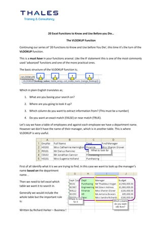
- 1. 20 Excel Functions to Know and Use Before you Die… The VLOOKUP Function Continuing our series of ‘20 Functions to Know and Use before You Die’, this time it’s the turn of the VLOOKUP function. This is a must have in your functions arsenal. Like the IF statement this is one of the most commonly used ‘advanced’ functions and one of the more practical ones. The basic structure of the VLOOKUP function is; 1 2 3 4 Which in plain English translates as; 1. What are you basing your search on? 2. Where are you going to look it up? 3. Which column do you want to extract information from? (This must be a number) 4. Do you want an exact match (FALSE) or near match (TRUE). Let’s say we have a table of employees and against each employee we have a department name. However we don’t have the name of their manager, which is in another table. This is where VLOOKUP is very useful. First of all identify what it is we are trying to find. In this case we want to look up the manager’s name based on the department name. . Then we need to tell excel which table we want it to search in. Generally we would include the whole table but the important rule is: Written by Richard Harker – Business Systems Training Consultant
- 2. The text or value you are basing your search on MUST be in the left hand column of your look-up table. Our formula then in this case would be; =VLOOKUP(C2,$H$2:$J$7,2,FALSE) Note that we are cross-referencing with column 2 in the formula even though the information is in column I, because column I is the second column in our selected data range. Excel will automatically look in the left hand column of the selected look up range (this can be in the same workbook or a completely different one). Unfortunately, you cannot tell it to look anywhere else when using VLOOKUP. Notice in the example above, I am ignoring the DeptCode column and starting my selection from column H where the department names are listed. If you don’t do this…it simply will not work because it will never find ‘Finance’ in column G. In the event that there is no matching information returned from the VLOOKUP, you will get an #N/A error message appear in the cell. So far, we have searched for information based on an exact match which probably is the most likely way you will be using this function, but what if you want a near match? You’d think that simply typing in TRUE would do it, but you need to do one thing before finding near matches – sort your look up data in ascending order. Depending on the version of Excel you have, you may get different results but this will guarantee that you get the correct result. If Excel cannot find an exact match, it will search for a value higher than the one you are looking for and then will select the previous cell and return that as the nearest match. All of the above techniques will of course apply to HLOOKUP, where instead of searching down columns it will search along rows although the most likely scenario is that you will be using VLOOKUP as most data is set up in vertical lists/tables rather than horizontal ones. Once you have mastered VLOOKUP, cross matching data across worksheets and even workbooks will become a breeze and will save you a lot a manual data entry which you are probably doing at the moment if you are not yet using the ‘must know’ VLOOKUP. Next time in this series……a bunch of statistical functions. Written by Richard Harker – Business Systems Training Consultant